Visual Sky Radar
Distributed multi-camera system for real-time aerial tracking
- Role
- Solo — concept, software, calibration, field testing
- Duration
- 2025, ongoing
- Team
- Solo
- Tools
- C++17, Qt6, OpenCV, FFmpeg, Python
Two cameras, one shared patch of sky
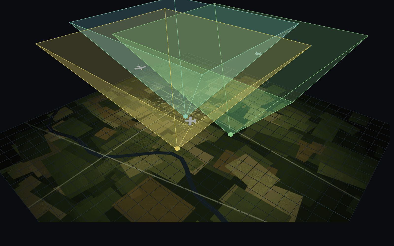
Every detection and triangulation is validated in a simulated 3D environment before it runs on real hardware: ground cameras with known positions and orientations watch simulated aircraft cross their overlapping fields of view. Drag the model to look around.
Recreation of the simulation environment: two to three ground cameras with overlapping fields of view over satellite terrain, tracking aircraft crossing the shared airspace.
Can two cheap phone cameras triangulate an aircraft?
Every plane overhead already broadcasts its position over ADS-B — services like OpenSky make that data public. But I wanted to know whether I could independently see and locate aircraft myself, from the ground, using nothing but two ordinary phone cameras and some geometry.
The goal: point two fixed, calibrated cameras at the sky from two different locations, detect the same aircraft (or its contrail) in both feeds, and triangulate a 3D position — then cross-check it against the real ADS-B track for that flight.
Two ground stations, one triangulated track
The system began as two independent camera stations roughly 4.3 km apart, and now runs three. Each station watches its own slice of sky, detects candidate targets locally, and reports a bearing — azimuth and elevation — toward anything it finds. No station ever sends video anywhere; what crosses the network is a handful of angles per detection.
Where two bearings from two known locations cross, that intersection is a 3D position estimate — classic optical triangulation, just aimed upward instead of across a lab bench. The baseline between the stations is what makes it work: the wider the separation, the sharper the angle at which the two lines of sight meet, and the better conditioned the intersection.
That same geometry sets the error behaviour, and it is worth being clear about it. Bearing error translates into position error roughly in proportion to range, so a fixed angular uncertainty that is worth metres at close range is worth hundreds of metres at cruise altitude and slant range. And when a target sits near the plane containing both cameras, the two bearings become nearly parallel — the intersection stretches out along the line of sight and the depth estimate degrades badly, even though each individual bearing is as accurate as ever.
Almost every refinement further down this page exists to attack one of those two error sources: sharpen the bearings, or improve the geometry they are intersected in.
Recreated schematic from camera_specs.json — real FOV and baseline geometry, redrawn (site does not include on-site photos yet).
Turning a phone camera into a measuring instrument
A phone's stated field of view is a marketing number, not a calibration certificate — I needed the real horizontal and vertical FOV of each sensor, in its actual mounted orientation, to trust any angle I derived from a pixel position.
I measured it the direct way: camera fixed at a known distance from a flat wall marked at even intervals, sighting the extreme visible marks and solving the subtended angle from simple trigonometry. That gave real fov_horizontal_deg / fov_vertical_deg values per camera — 34.0°×57.0° for one unit, 35.6°×58.2° for the other — which now live in the app's camera_specs.json as the source of truth for every bearing calculation downstream.
Each camera also needed a yaw/tilt orientation ('cone' in the code) so its pixel grid maps onto real compass bearings and elevation angles — set once during setup and stored in cone_orientations.json.
Recreated schematic of the wall-calibration method — sighting evenly spaced marks at a measured distance to solve for each camera's true horizontal/vertical field of view.
Finding a thin white line in a noisy blue sky
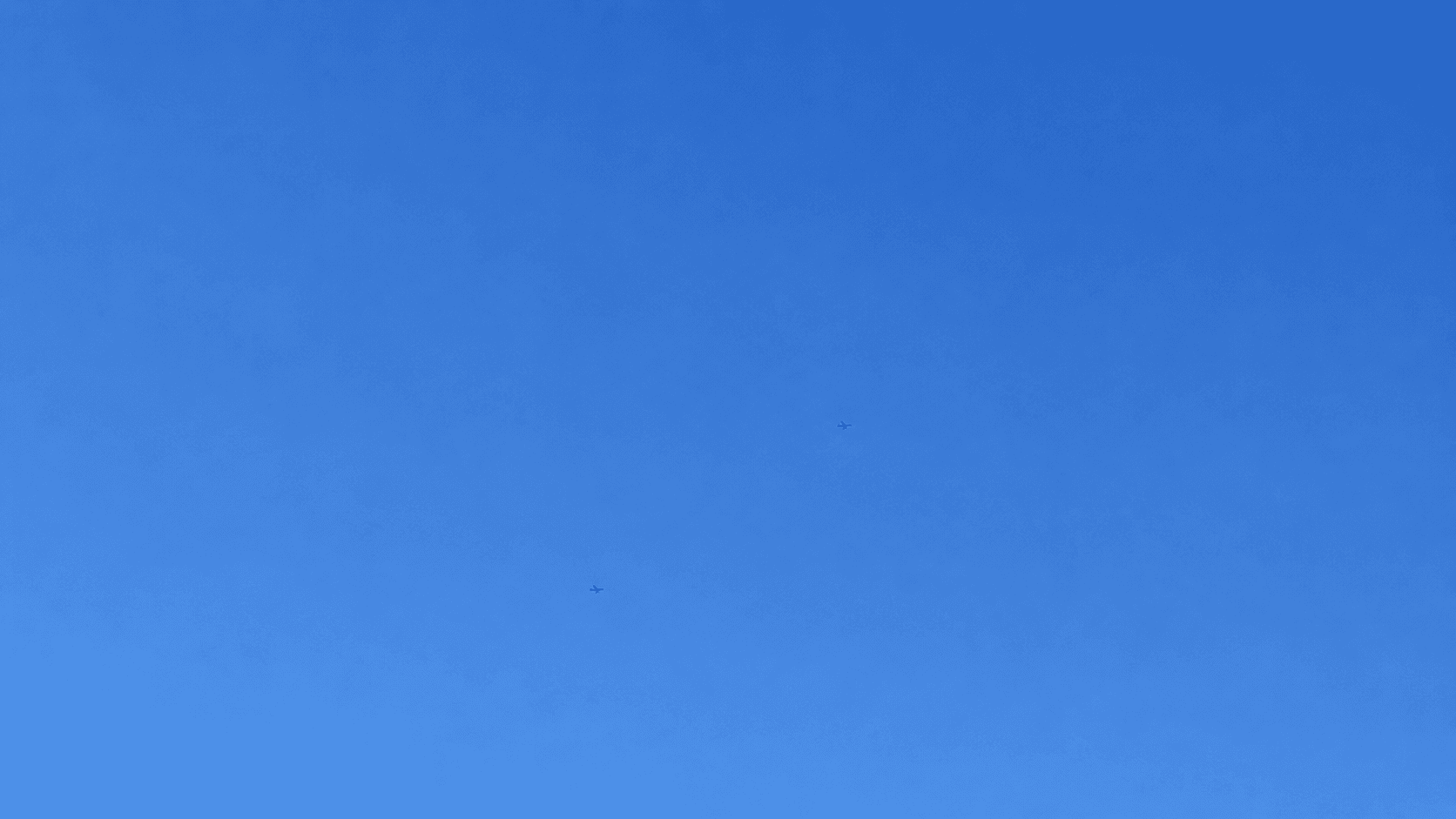
A contrail is a faint, thin, high-contrast streak against a sky that has its own gradients, sensor noise, and JPEG artefacts. A naive brightness threshold picks up compression noise as readily as an actual contrail — so detection became a staged pipeline, each stage narrowing down what's left.
Bright-region extraction → sky masking → edge detection → frame-to-frame motion → morphological top-hat filtering to isolate thin linear structures → dark-sky suppression → line-bank scanning to confirm a real elongated streak rather than a blob of noise.
Every stage is independently visualised during development, which made it possible to see exactly where a false positive was entering the pipeline instead of just staring at a final yes/no.
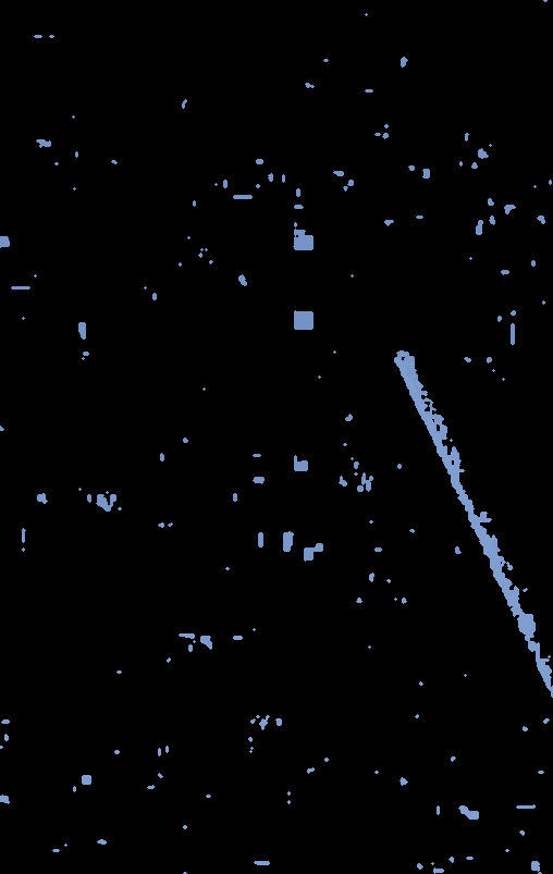
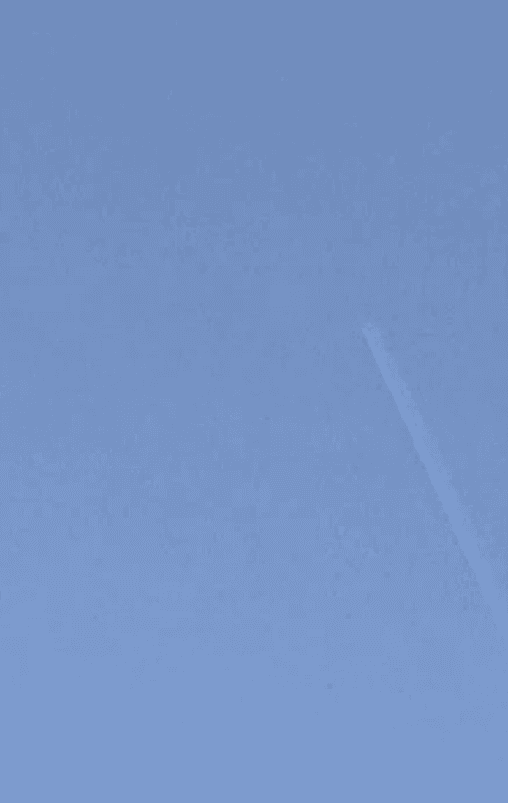
Sweeping parameters until the noise disappears
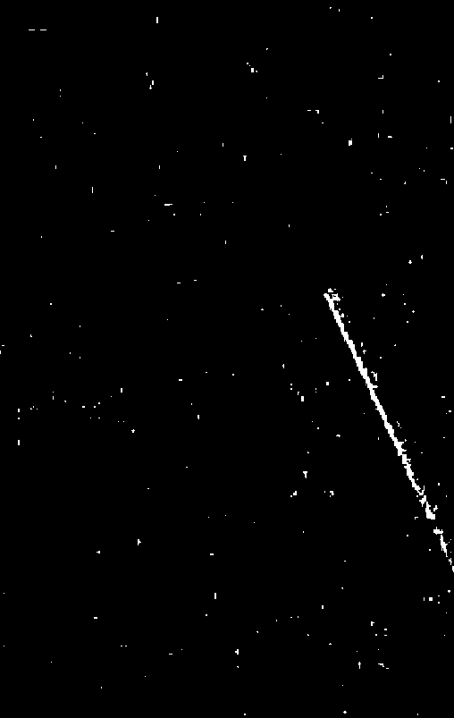
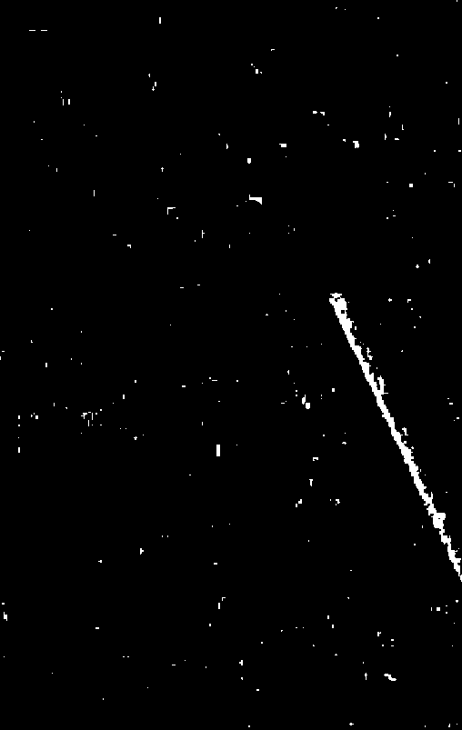
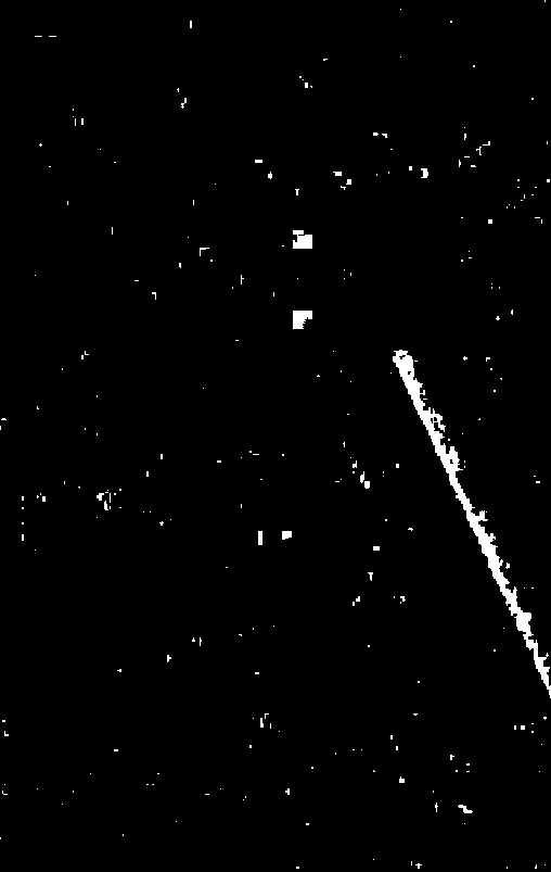
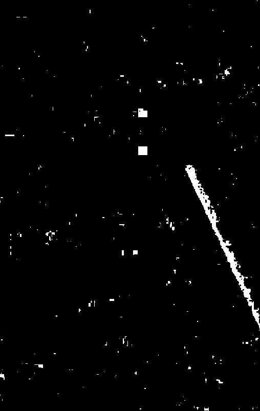
Each stage has a free parameter or two — the Gaussian brightness sigma, the morphological kernel size, the line-opening length — and none of them have an obvious 'correct' value on paper. I swept them systematically against real recorded footage and compared outputs side by side.
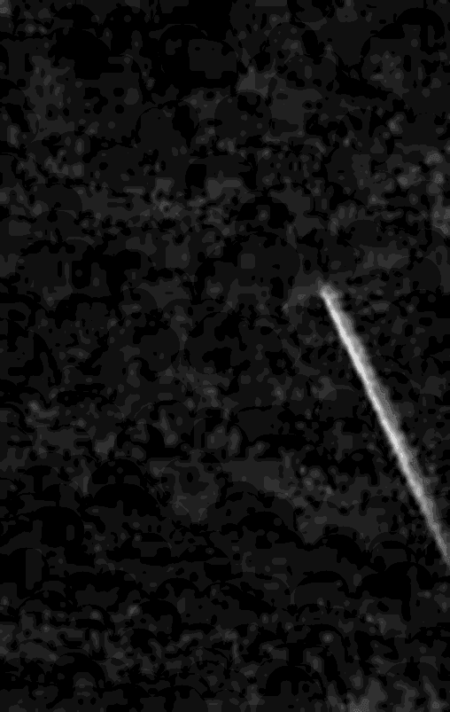
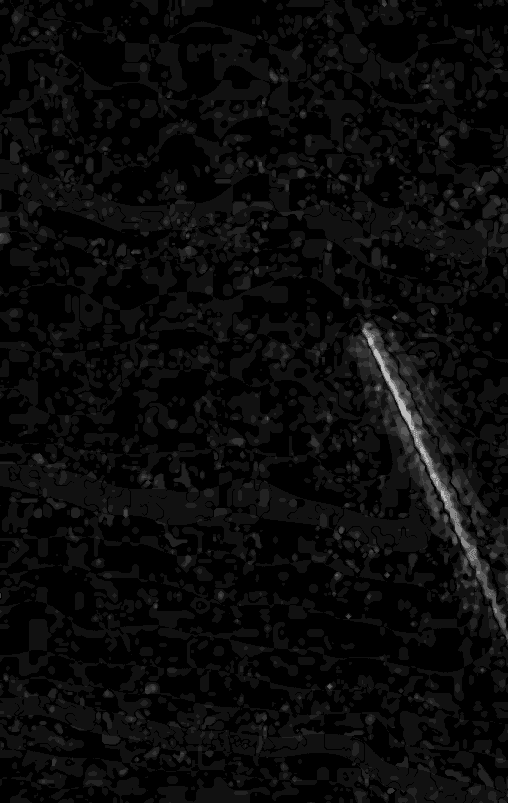
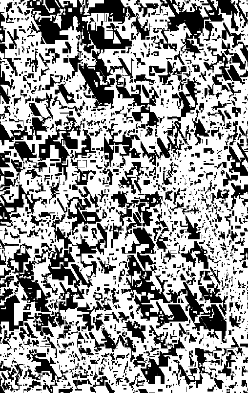
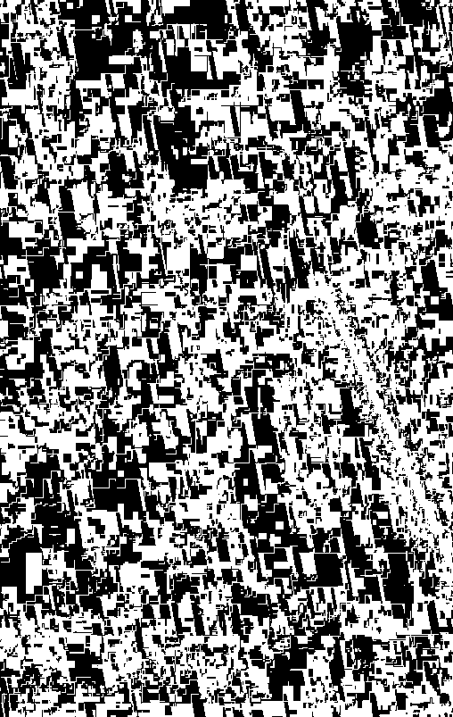
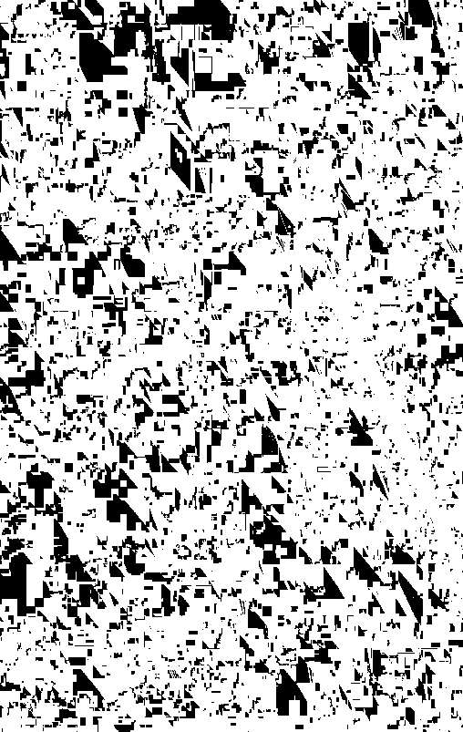
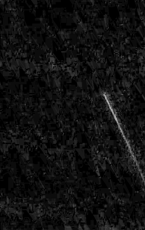
Below: the same brightness-extraction stage at four different sigma values. Too small and the contrail fragments into noise; too large and it smears into the surrounding sky gradient. The working value sits in a narrow band in between — the kind of thing you only find by testing, not by deriving.
A bank of line detectors, not a single threshold
The last confirmation stage runs a bank of directional line-opening filters at different lengths and orientations, then combines them — a single filter length either missed short contrail segments or let short noise streaks through, so I settled on running several in parallel and taking their union.
Testing without waiting for a plane to fly over
Real contrail sightings are intermittent and weather-dependent, which is a miserable feedback loop for iterating on a detector: change a parameter, then wait for the sky to cooperate before finding out whether it helped.
So I built synthetic feeds — generated frames with aircraft and contrail shapes injected at known positions, on known trajectories, over backgrounds with controllable noise and sky gradient. That inverts the problem. Instead of guessing whether a missed detection was the detector's fault or the weather's, I know exactly what was in the frame and exactly where, so every miss and every false positive is attributable.
It also makes the detector's failure boundary measurable rather than anecdotal. Sweeping contrail contrast down until detection breaks gives a real answer to "how faint can it be and still be found", which is not a question intermittent real sightings can answer in any reasonable amount of time.
The synthetic feeds carry the obvious caveat that they only contain the failure modes I thought to simulate — real skies produce cloud edges, lens flare and aircraft that are nothing like the model. They are for fast iteration; the real footage remains the judge.
From research script to a live Qt6 application
The working pipeline moved from a Python prototype into a native C++17 / Qt6 application with FFmpeg-based RTSP ingestion, so it can run continuously against live camera feeds rather than pre-recorded clips. The Python side still hosts the terrain-cache rendering, OpenSky polling, and the analysis tooling used to validate results.
Each station's FOV calibration and cone orientation live in versioned JSON config files — camera_specs.json and cone_orientations.json — so re-pointing or re-calibrating a station doesn't require touching code, just re-running the wall calibration and updating a couple of numbers.
Adding a third camera to break the ambiguity
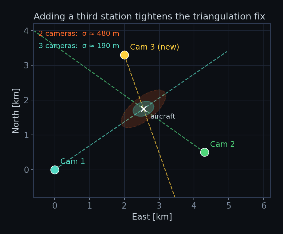
Two stations fix a target where their bearings cross, but that intersection is only as sharp as the angle between them. When an aircraft sits near the line joining the two cameras, the fix smears out along the line of sight and the depth estimate becomes almost meaningless.
I added a third station, offset from the 4.3 km baseline of the first two, so every point in the shared airspace is now seen from three well-separated directions. The redundant bearing removes the near-baseline ambiguity and enables outlier rejection: if one camera disagrees with the other two, the fix is still solved from the remaining pair.
On the same simulated pass, the 1-σ horizontal uncertainty at the crossing point drops from roughly 480 m with two cameras to about 190 m with three.
Calibrating out the residual angle offsets
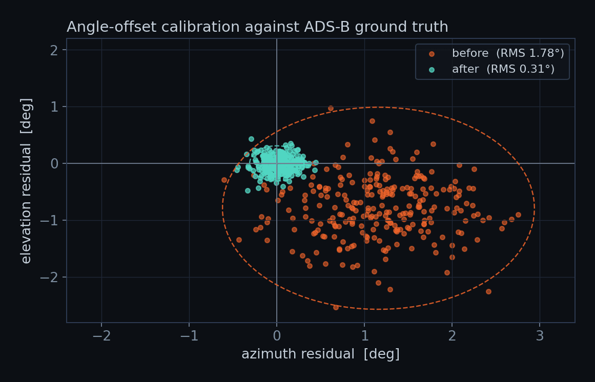
Even with each camera's field of view measured against the wall, small mounting errors remain — a fraction of a degree of yaw or tilt that the setup procedure can't catch. Over a few kilometres of range, half a degree is tens of metres of position error, so those residual offsets had to go.
Instead of re-surveying the mounts, I let the aircraft calibrate the cameras: for every detection I could match to a known ADS-B track, I computed the bearing the camera should have reported and compared it to the bearing it did report. Fitting a constant azimuth/elevation offset per camera that minimises those residuals across hundreds of matched detections pins the misalignment down directly in the coordinate frame that matters.
After applying the fitted offsets, the bearing-residual RMS collapsed from about 1.78° to 0.31° — most of what's left is genuine detection noise rather than a fixed pointing bias.
A Kalman filter to fuse motion with noisy fixes
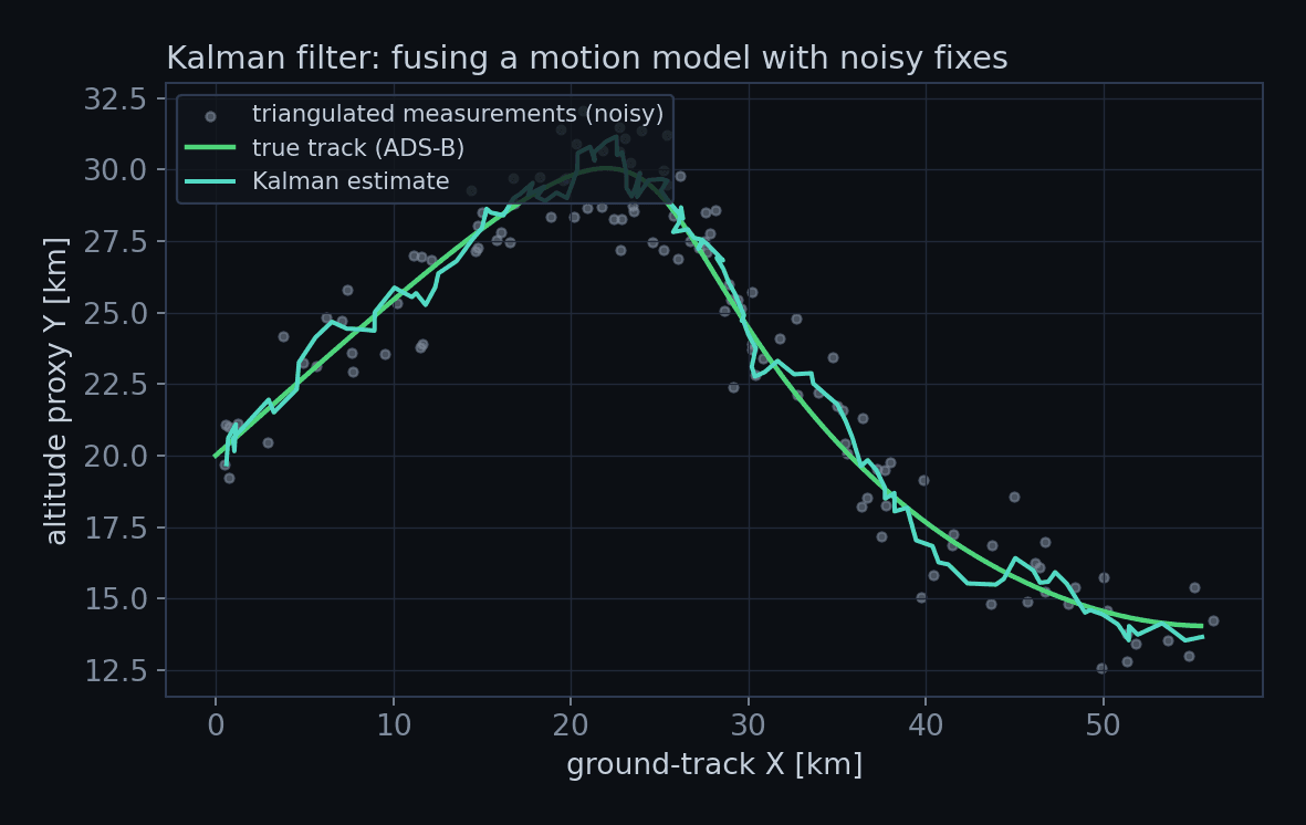
A raw triangulated position jumps around from frame to frame — each fix carries a metre or two of bearing noise, and a plain frame-by-frame track looks like a scatter plot. But an aircraft doesn't teleport; it flies a smooth, roughly constant-velocity path, and that prior is information worth using.
I introduced a constant-velocity Kalman filter that carries a position-and-velocity state: it predicts where the target should be on the next frame from its motion model, then corrects that prediction with the incoming triangulated measurement, weighting the two by their relative uncertainty. The track stays smooth through noisy fixes and coasts sensibly through the occasional dropped detection.
Going unscented for the nonlinear geometry
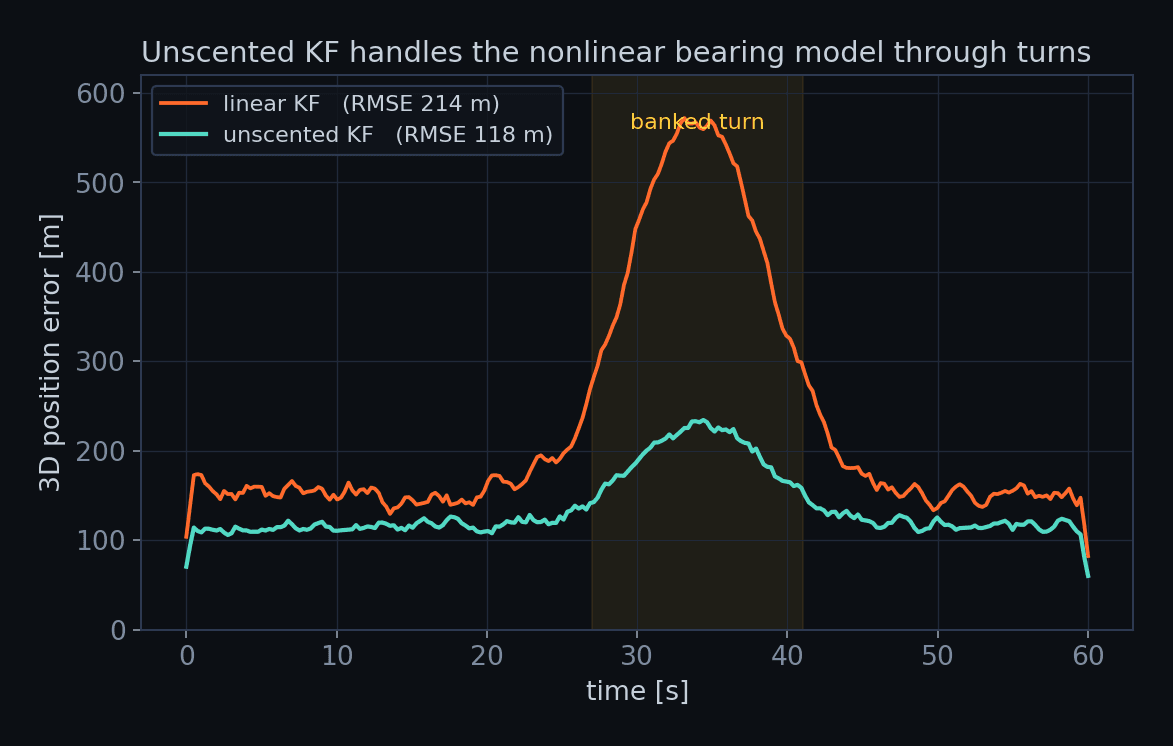
The linear Kalman filter fuses positions cleanly, but the actual measurements aren't positions — they're bearings, and the map from a 3D position to a pair of camera angles is distinctly nonlinear. Linearising it around the current estimate is fine while the target flies straight, but through a banked turn the linearisation error grows and the filter lags and overshoots.
So I swapped the linear update for an Unscented Kalman Filter: instead of linearising, it propagates a small set of deterministically-chosen sigma points through the true nonlinear bearing model and reconstructs the mean and covariance from where they land — capturing the curvature the linear filter throws away.
Across a scripted trajectory with a mid-pass turn, 3D position RMSE dropped from about 214 m with the linear filter to 118 m with the UKF, and the error spike through the turn itself shrank from roughly 560 m to 230 m.
A three-station, filtered tracking pipeline
The system now runs three calibrated ground stations, detects contrails and bright aircraft across a range of sky conditions, and cross-references every detection against live ADS-B traffic. Residual pointing offsets are calibrated out against matched tracks, and triangulated fixes are fused through an unscented Kalman filter into a smooth 3D track that holds up through turns and dropped frames.
Measured against the original question — can two cheap phone cameras triangulate an aircraft — the answer is yes, with the caveat that the interesting work was never the triangulation. Intersecting two bearings is trigonometry. Everything that took real effort went into making those bearings trustworthy: calibrating fields of view that the manufacturer states only approximately, fitting out the residual mounting misalignment against ADS-B truth, and rejecting the enormous number of things in a sky photograph that look like a thin white line and are not an aircraft.
The current frontier is timing. Bearings fused at a given instant have to belong to the same instant, and three independent cameras with independent capture clocks do not naturally agree on when "now" is. A target crossing the sky moves measurably between frames, so a synchronisation error of a fraction of a second injects a bearing error that no amount of filtering removes — it looks like a consistent, plausible measurement of a position the aircraft was not at. That is the largest remaining source of triangulation error and the next thing to fix.
After that, the obvious extension is to let the system use its own history: the ADS-B cross-reference currently validates tracks after the fact, but the same matched data could train the detector on exactly the targets it missed.