Comparison of Turbulence Models in Sub- and Transonic Flow

Every RANS simulation stands or falls with its turbulence model — and every CFD engineer eventually faces the same question: which one should I trust for this flow? This project, from the CFD application seminar (CFD-Anwendungsseminar) at the University of Stuttgart's Institute of Aerodynamics and Gas Dynamics (IAG), answers it the empirical way: run the same airfoil through six turbulence models and compare everything — pressure distributions, force coefficients, shock positions, convergence behaviour and computing time — against wind-tunnel truth.

The test article is the RAE 2822, a classic transonic research airfoil with an extensive experimental database (AGARD-AR-138). Two of its documented wind-tunnel cases span the interesting range: Case 1, subsonic at Mach 0.676, Re = 5.7 million and α = 1.92°, and Case 9, transonic at Mach 0.73, Re = 6.5 million and α = 2.78° — the latter with a shock sitting on the upper surface, which is exactly where turbulence models start to disagree.

The contenders cover the whole ladder of RANS closure complexity: two one-equation models (Spalart-Allmaras original and with Edwards modification), three two-equation models (k-ω, Menter Baseline and Menter SST), and a full Reynolds-stress model that solves a transport equation for every component of the stress tensor. All simulations ran in the DLR TAU code on meshes built in Pointwise, and beyond the two validation cases the models were pushed through full polar sweeps up to and past maximum lift — where the comparison got dramatic.

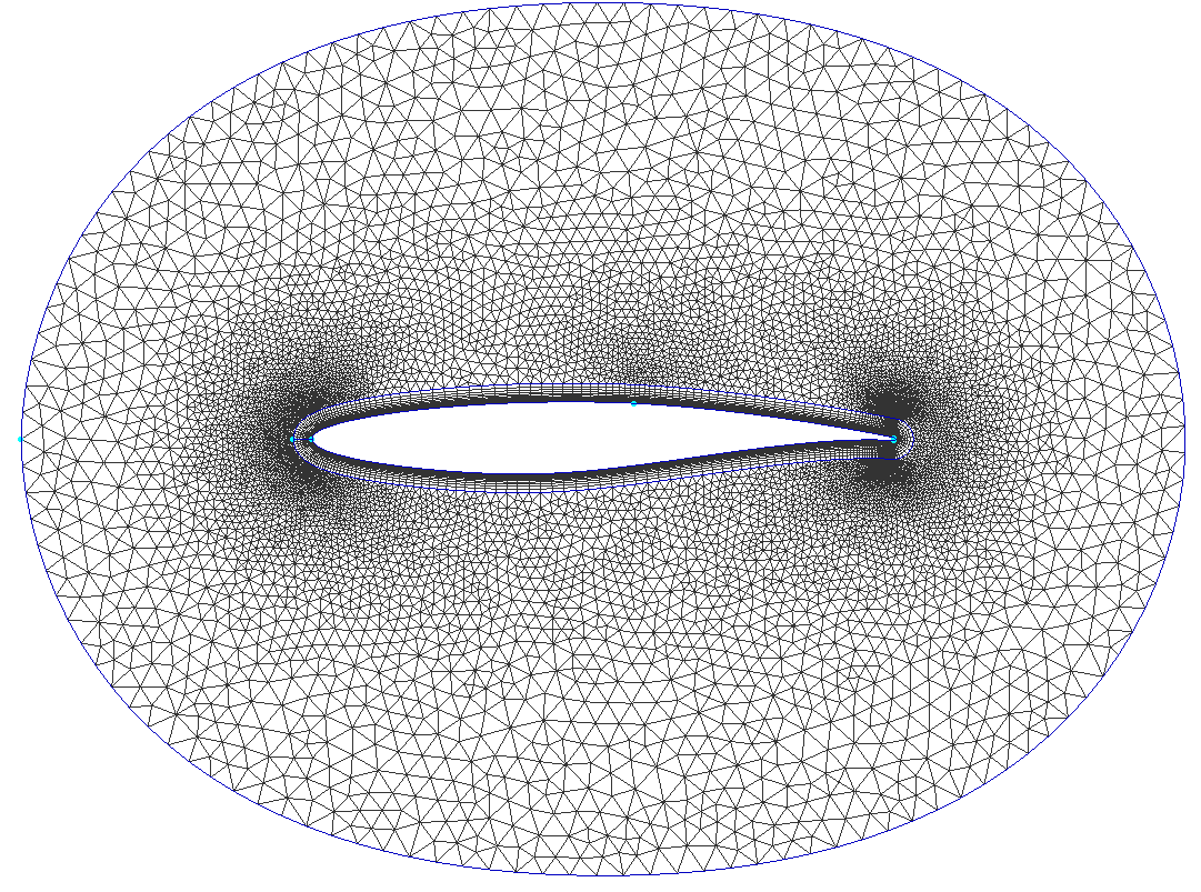
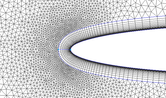
The mesh is hybrid, built in three parts: a structured block hugging the airfoil to resolve the boundary layer, and two unstructured rings filling the space out to circles of one and eighty chord lengths. Surface point distributions are pinned by spacing constraints at the leading and trailing edges, and the first cell height is set via the y⁺ target — between 0.3 and 1.0 depending on resolution — so the boundary layer is genuinely resolved rather than bridged with wall functions.

The transonic case got special treatment. A shock smeared over a coarse region contaminates every coefficient downstream of it, so its location was found first with a precursor run on the unrefined mesh — the intersection of the computed pressure distribution with the critical pressure coefficient marks where the flow goes supersonic and where it recovers — and the mesh was then refined there. The inner refinement circle was also squeezed into an ellipse (two chords long, one and a half high) to concentrate cells around the profile and its shock instead of wasting them above and below.

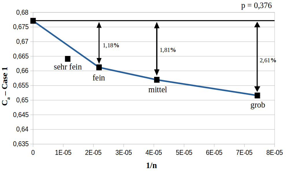
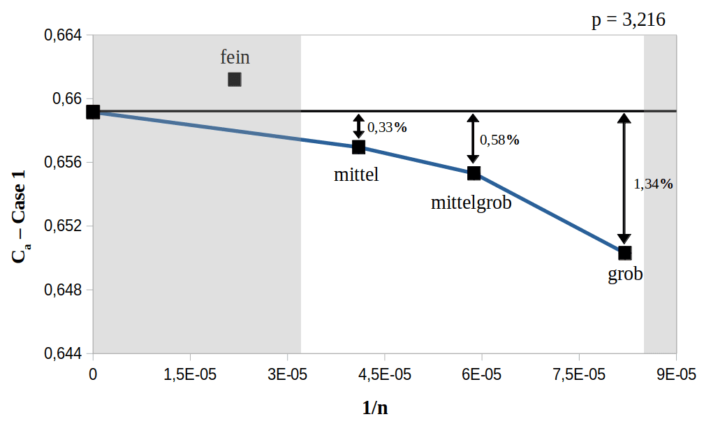
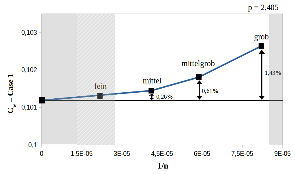
Before comparing turbulence models, the discretisation error has to be pinned down — otherwise model differences and mesh artefacts blur together. The tool is Richardson extrapolation: run the same case on systematically refined meshes (total cell count doubling each step), fit the observed convergence order, and extrapolate to the value an infinitely fine mesh would produce. The distance of each mesh from that limit is its error estimate.

The first attempt failed instructively. With the coarse, medium and fine meshes the fitted convergence order came out at p = 0.376 — far below the theoretical order of the scheme — because the fine mesh had already left the asymptotic range: its discretisation error was small enough that round-off and iteration error started to dominate, bending the curve the wrong way. More cells were actively hurting.

The fix was to move the study window coarser instead of finer: a new intermediate mesh (scaling factor √1.5, dubbed 'mittelgrob') and a rebuilt coarse mesh with a matched refinement ratio. With that triplet the lift coefficient converged with p ≈ 3.2 and the drag coefficient with p ≈ 2.4, both cleanly asymptotic. The medium-coarse mesh — about 17,000 nodes, 0.58% lift error and 0.61% drag error against the extrapolated limit — was chosen for all following comparisons: accurate enough that model differences dominate, cheap enough to run six models through full polar sweeps.

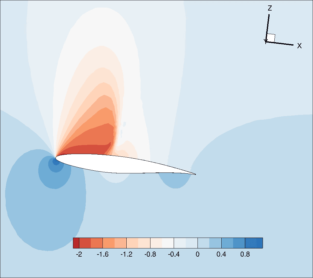
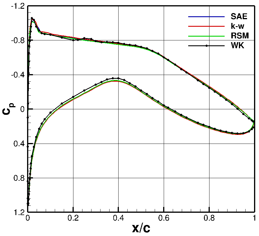
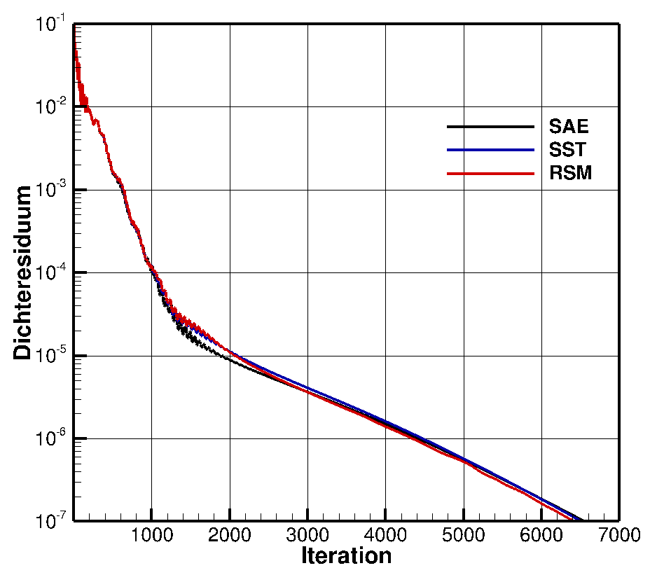
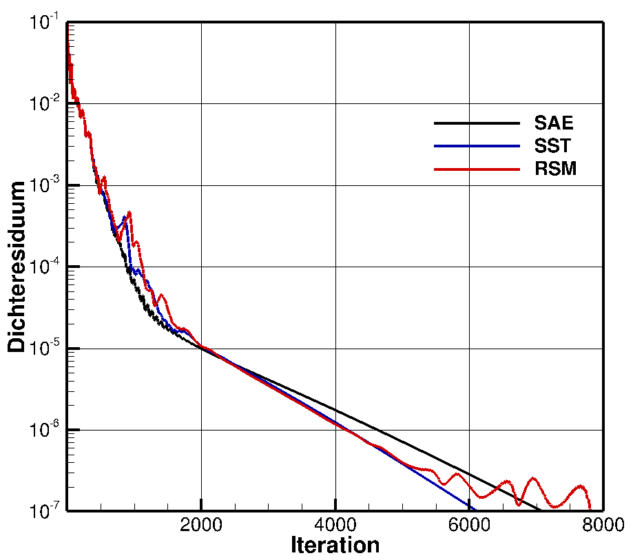
At Mach 0.676 and low incidence the flow stays attached and shock-free, and the models behave accordingly: all six pressure distributions lie practically on top of each other, matching the wind-tunnel curve through the suction peak and across the whole upper surface. Every model converged steadily to a density residual of 10⁻⁷ without drama. If this were the whole story, the cheapest model would win by default.

The one systematic deviation isn't a model's fault. On the lower surface the measured pressure sits visibly below every simulation — consistent with wind-tunnel blockage: the model narrows the test-section cross-section, the flow accelerates around it, and the pressure drops per Bernoulli. The same offset shows up in the integral coefficients: all simulations cluster between lift coefficients of 0.577 and 0.598 while the tunnel reports 0.566, and the computed drag (95–100 counts) sits above the measured 85 counts for the same reason.

The spread between the models themselves stays small — the two-equation k-ω is highest at 0.598, Menter SST lowest at 0.577 — a first hint of the pattern the transonic case would amplify.

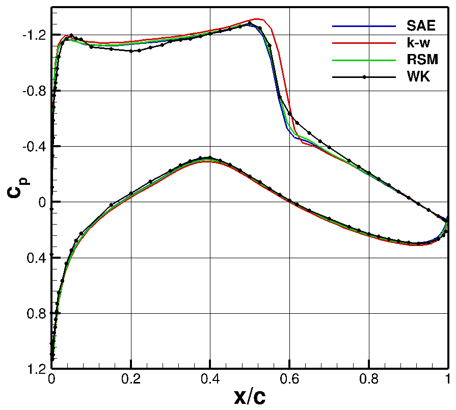
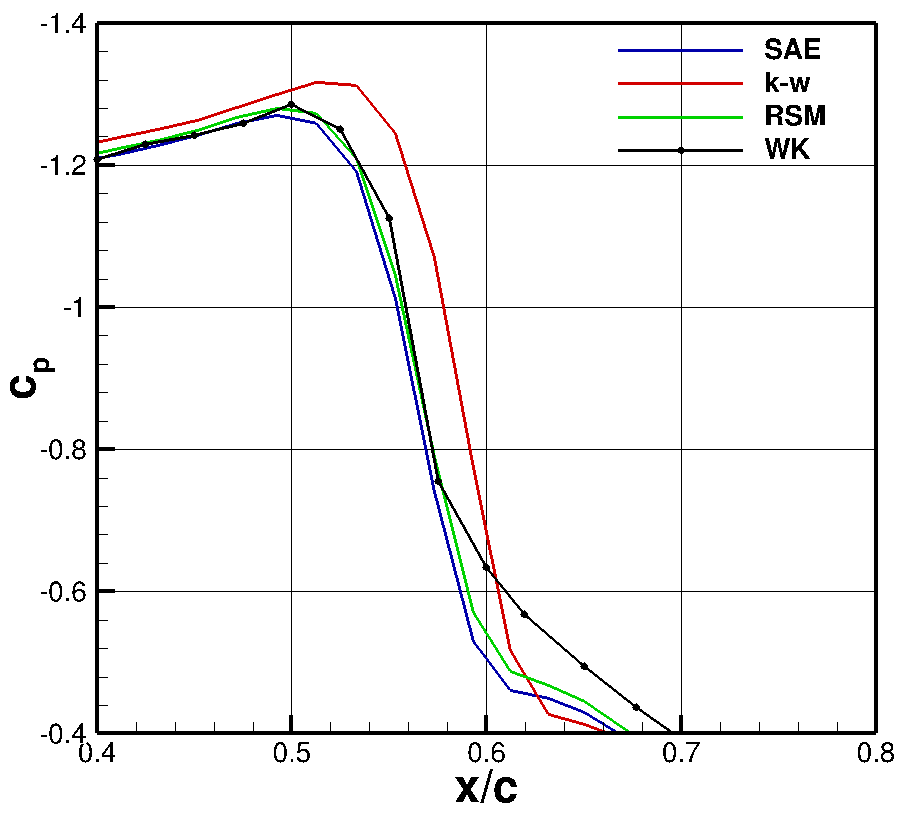
At Mach 0.73 a supersonic pocket forms on the upper surface and collapses through a shock at mid-chord — and now the models diverge exactly where the physics gets hard. The shock position was extracted objectively from each solution as the intersection of the pressure distribution with the critical pressure coefficient. The one-equation Spalart-Allmaras variants and the Reynolds-stress model all place the shock at x/c ≈ 0.56, in close agreement with the wind tunnel. The k-ω model puts it a full two percent chord too far downstream at 0.58 — its known habit of predicting separation and shock positions too far aft — and Menter Baseline, which is k-ω near the wall by construction, lands at the same spot.

Menter SST shows precisely the behaviour it was designed for: its eddy-viscosity limiter pulls the shock back upstream to x/c ≈ 0.55 — overcorrecting slightly to the early side, but much closer than its k-ω base. The integral coefficients tell the same story: k-ω's late shock enlarges the suction area and inflates lift to 0.847 against the tunnel's 0.803, while SAO (0.800), SAE (0.801) and the RSM (0.814) land close, and SST sits slightly low at 0.788.

The transonic case also cracked the first model's composure: the Reynolds-stress model's residual, smooth in the subsonic case, starts oscillating visibly on its way down — it still converges, but the reduced numerical robustness the literature promises is now on screen.

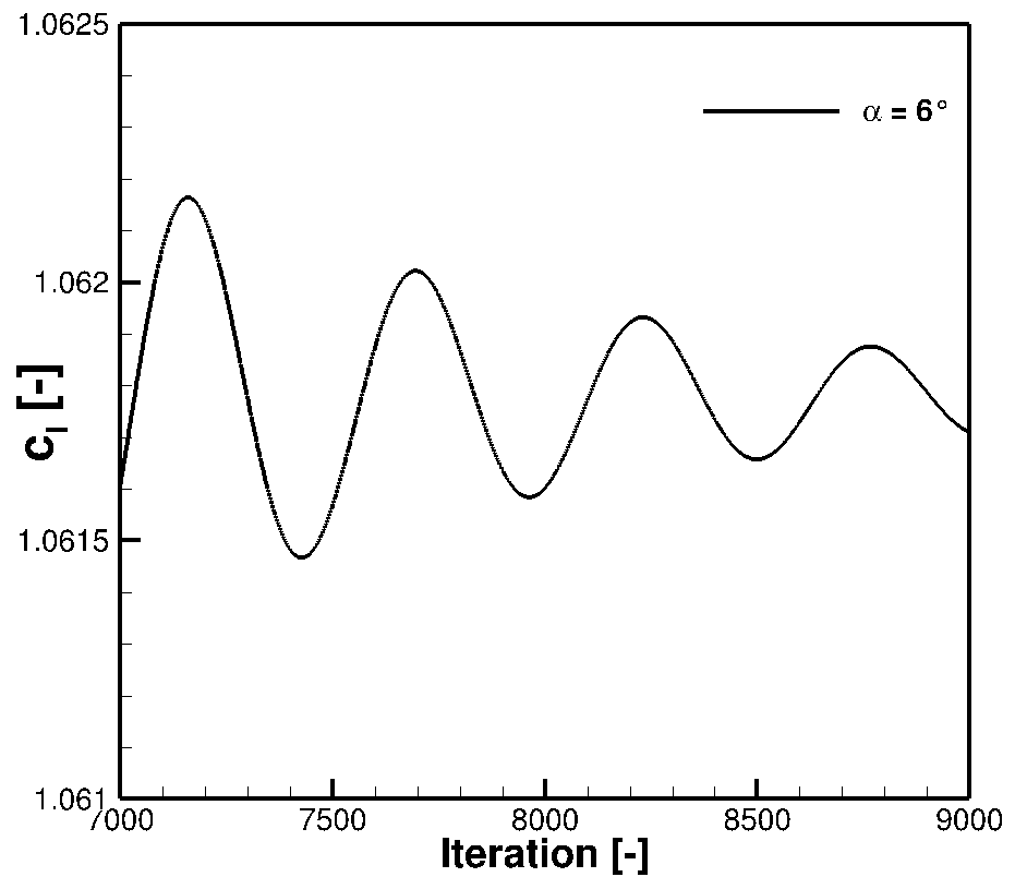
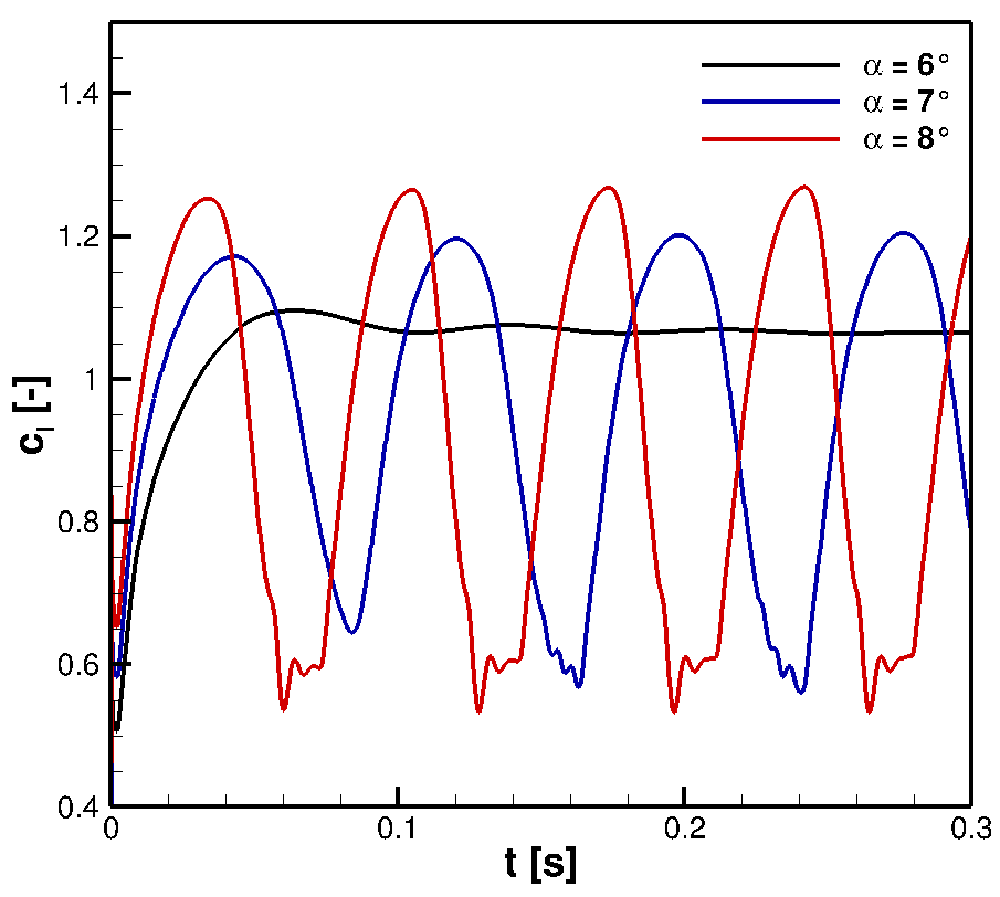
The wind-tunnel cases live below α = 3°, where every model behaves. The polar sweeps — flown with one representative per family: SAE, Menter SST and the RSM — push into the regime where the solution itself becomes the problem. Above roughly six degrees the steady computations stop converging and the force coefficients start ringing: the residual oscillates instead of dropping, and the 'converged' lift value depends on where you stop iterating.

The remedy is honest time integration. In the unsteady runs two situations separate cleanly: at moderate incidence the lift coefficient still settles to a stable value, while at higher angles a genuine periodic oscillation develops that no amount of iteration will remove — the flow itself is unsteady. For those cases the coefficients entering the polar are time-averaged over the oscillation.

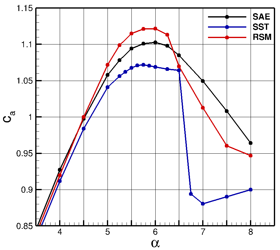
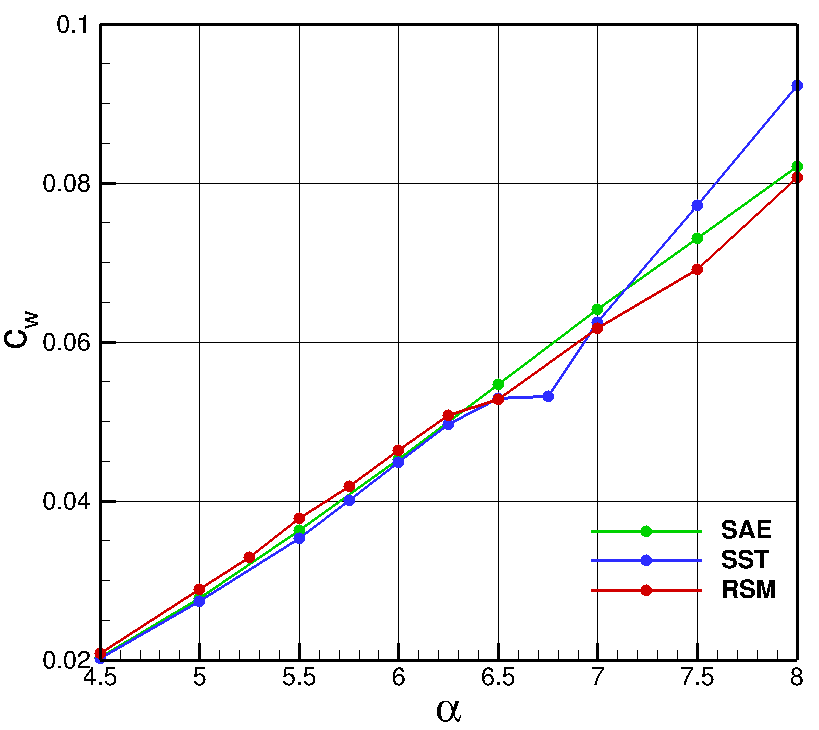
The resulting polars around maximum lift disagree far more than any low-α result: SAE traces the textbook shape — a rounded lift peak of about 1.10 at six degrees with boundary-layer thickening, separation and stall discernible in the drag curve. The RSM carries the highest maximum lift, about 1.12. And Menter SST does something neither of the others does: after 6.5° its time-averaged lift collapses by nearly 0.2 within a quarter of a degree, with a matching kink in the otherwise linear drag curve. That cliff has a specific cause — the next chapter watches it happen.

Zooming into the two computations bracketing the cliff — α = 6.5° and 6.75° with Menter SST — reveals a shock buffet: the shock is no longer stationary but sweeps periodically across the upper surface, oscillating between roughly 4% and 56% chord. Each cycle the supersonic pocket builds, collapses, sheds and rebuilds; the animations of the Mach and pressure fields show the whole breathing motion.

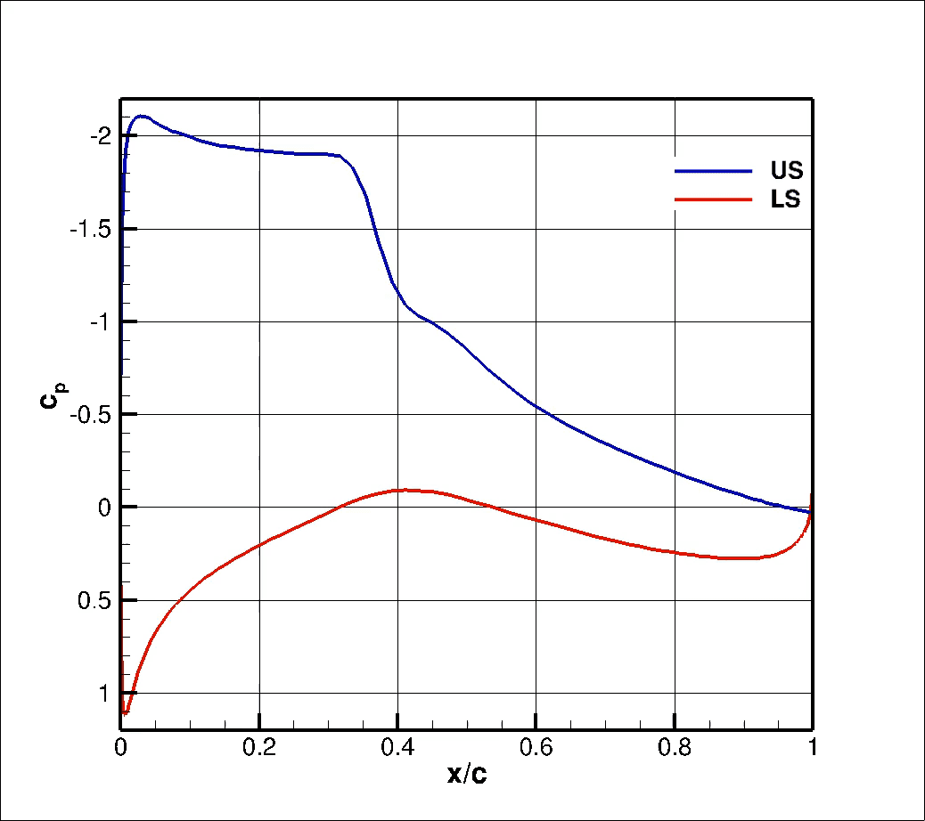
The surface pressure explains where the lift goes. At the low point of each cycle the upper- and lower-surface pressure distributions cross over the rear part of the airfoil — the aft loading reverses sign, the rear of the airfoil briefly lifts downward, and the instantaneous lift dips far below its shock-quiet value. The lift coefficient still touches its former level once per period, but the time average — which is what the polar records — collapses. At 6.5° the curves never cross and the polar stays intact; a quarter degree later they do.

This is exactly the flow situation the summary tables warn about with 'convergence problems in separated flow' — experienced live: SST's limited eddy viscosity, the very mechanism that fixed the shock position in Case 9, also makes it the first model to let the shock start moving.

At seven degrees all three models agree the flow is unsteady — and disagree on almost everything else about it. Side by side, the pressure-field animations show three different renditions of the same buffet: the Spalart-Allmaras model oscillates with a period of 73 ms, Menter SST slowest at 78 ms with the largest excursions and the most chaotic field, and the Reynolds-stress model fastest at 64 ms.

This is the sobering endnote of the comparison: in exactly the regime where a designer would most want a trustworthy answer — buffet onset, the boundary of the safe flight envelope — the models diverge not by percent but qualitatively, in amplitude, frequency and character of the unsteadiness. Below buffet onset any of them would do; at it, the model choice is the answer.