Enhancing Spacecraft Thermal Design through Automated Data Correlation

Every spacecraft is thermally modelled long before it flies. A geometric mathematical model (GMM) captures the shapes, surfaces and view factors that govern radiation; a thermal mathematical model (TMM) turns that geometry into a network of nodes, conductances and heat capacities and predicts how the structure heats and cools through an orbit. Those predictions decide radiator sizing, heater power budgets and whether an instrument stays inside its qualification range — so the model is not a document, it is the design.

And the model is always wrong by some margin. Not because it is badly built, but because its inputs are genuinely uncertain: the emissivity of a surface after handling and ageing, the conductance across a bolted joint, the effective conductivity of a multi-layer insulation blanket, the radiative coupling between two units that see each other partially. These are not quantities anyone measures directly on the flight article. They are estimated, and estimates carry error.

The only way to find out how far off they are is to put the spacecraft in a thermal-vacuum chamber, drive it through representative hot and cold cases, and compare hundreds of measured thermocouple temperatures against what the model predicted for those same nodes.

Closing the gap between the two is called model correlation, and it is traditionally done by hand: a thermal engineer picks a handful of suspect parameters, nudges them, reruns the model, looks at the residuals, and repeats until the predictions sit within the required tolerance of the measurements. It works — correlated models fly — but it is slow, it depends heavily on the individual engineer's intuition about which parameters to touch, and it ends with a single set of tuned numbers that carries no statement of how confident anyone should be in them.

This thesis, carried out at Airbus Defence and Space, builds an automated and statistically grounded alternative, using Sentinel-2 as the real-world validation case.

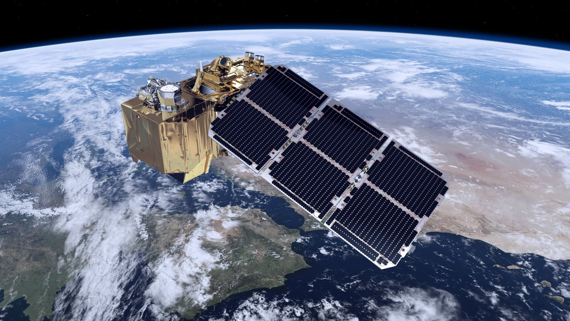
Sentinel-2 is an optical Earth-observation mission in the EU/ESA Copernicus programme, built by Airbus Defence and Space. Its thermal-vacuum test campaign produced the ground-truth temperature data this thesis correlates against — which makes it an unusually honest test case for a correlation method, because the right answer exists, was measured on real hardware, and was not generated by the same modelling assumptions the method is supposed to check.

Working from a real spacecraft model also means working at real scale. A flight-representative TMM is not a handful of nodes with three unknowns; it is a large thermal network whose correlation parameters number in the tens, spread across units, panels, joints and blankets, with sensors distributed unevenly across it. Some parameters are strongly observed by several thermocouples at once, and others are barely visible in the data at all. Any method claiming to automate correlation has to cope with that imbalance rather than assume it away.

The test data itself comes from the chamber: the spacecraft mounted in thermal vacuum, driven through steady-state hot and cold plateaus and the transients between them, with the thermocouple network logging throughout.

The change in approach is a change in the question being asked. Manual correlation asks: which single set of parameter values makes the model match the test best? The Bayesian formulation asks instead: given the test data, what do we now believe about each parameter, and how strongly?

That starts by treating every correlation parameter as a random variable rather than a number. Each one is given a prior distribution encoding what is known before the test is consulted — a plausible range for a contact conductance, a bounded interval for an emissivity — which is a more faithful description of the engineer's actual knowledge than a single hand-picked value ever was.

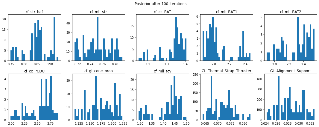
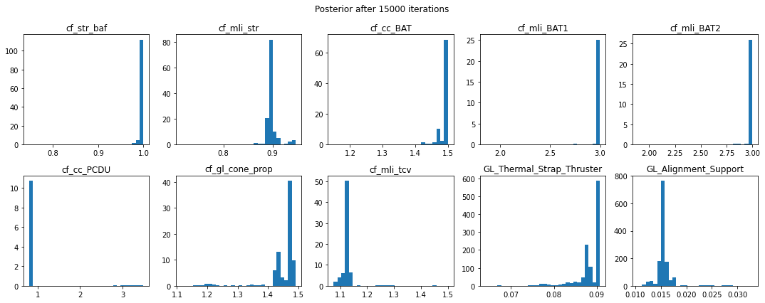
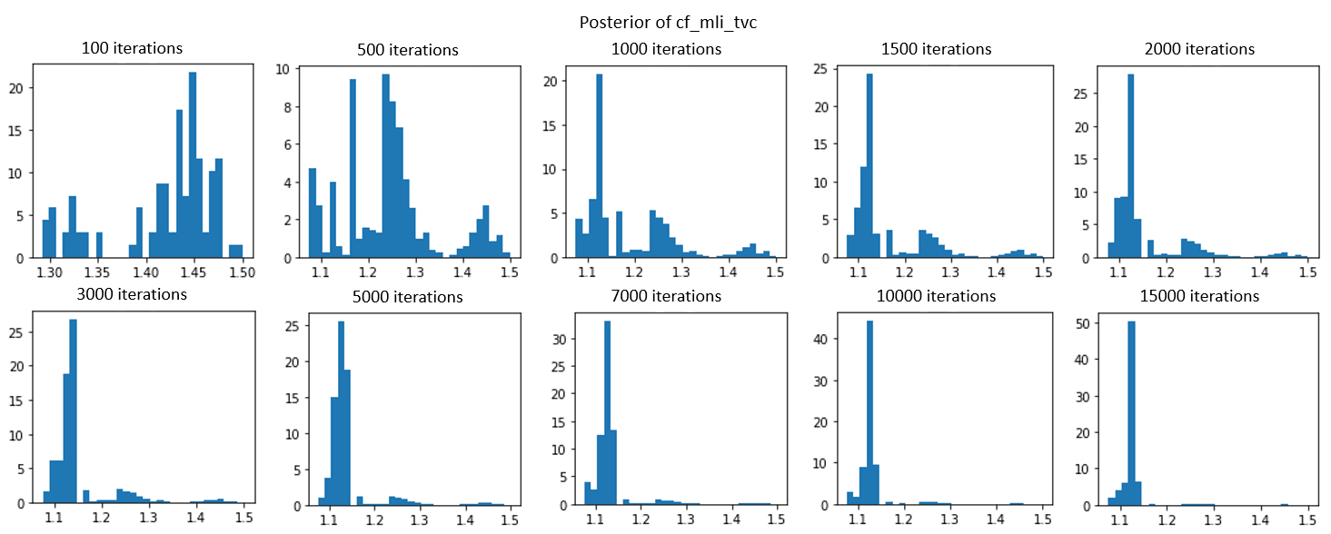
Markov chain Monte Carlo sampling then updates those priors against the measured chamber temperatures. The sampler proposes a parameter set, the thermal model predicts the sensor temperatures it would produce, those predictions are compared against the measurements through a likelihood function, and the proposal is accepted or rejected accordingly. Run long enough, the chain's accepted samples trace out the posterior — the distribution of parameter values consistent with the data.

The output is therefore not one number per parameter but a distribution per parameter, and the width of that distribution is as informative as its centre. Parameters the test data constrains tightly come out narrow and shifted away from their priors; parameters the sensors barely see stay close to their priors and stay wide — which is the method telling you, honestly, that this test campaign did not identify them and no amount of manual tuning would have made that untrue. It simply would have hidden it behind a confident-looking single value.

Correlations between parameters fall out of the same machinery. If two conductances can trade off against each other while producing the same temperatures, the posterior shows them as coupled rather than pretending each was determined independently.

There is a reason this is not already standard practice: MCMC is brutally expensive in model evaluations. Every proposed parameter set requires a full solve to produce predicted temperatures, and a converged chain needs tens of thousands of them. A flight-representative thermal solver takes far too long per run for that to be viable — the statistically correct method is, in its raw form, computationally impossible.

The way through is to stop calling the solver inside the loop. A neural network is trained to approximate the mapping the solver performs — correlation parameters in, node temperatures out — using a set of solver runs generated across the parameter space as training data. Once trained, it evaluates in a fraction of the time, and it is the surrogate, not the solver, that the sampler queries.

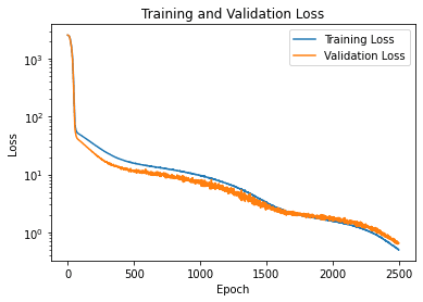
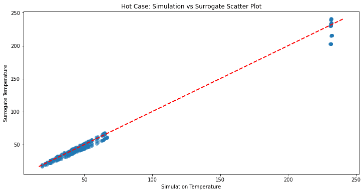
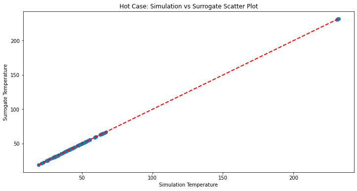
That only works if the surrogate is trustworthy, so it has to earn the substitution. Training is monitored for convergence and overfitting, and the trained network is then validated against solver runs it never saw during training — predicted temperatures plotted against true solver temperatures, where a perfect surrogate lies on the diagonal and the scatter around that line is the error being introduced into every subsequent inference.

This is the pivotal engineering judgement in the whole pipeline. Surrogate error propagates directly into the posterior: too loose, and the distributions describe the network's quirks rather than the spacecraft's physics. The scatter plots below are the evidence that the approximation is tight enough for the substitution to be legitimate.

Not every parameter deserves to be in the inference. In a large thermal model most parameters barely move most sensors, and carrying them through sampling costs dimensions — and MCMC gets rapidly harder as the parameter space grows.

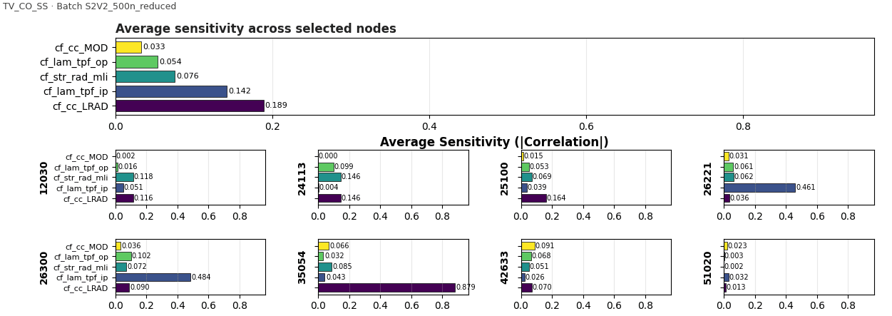
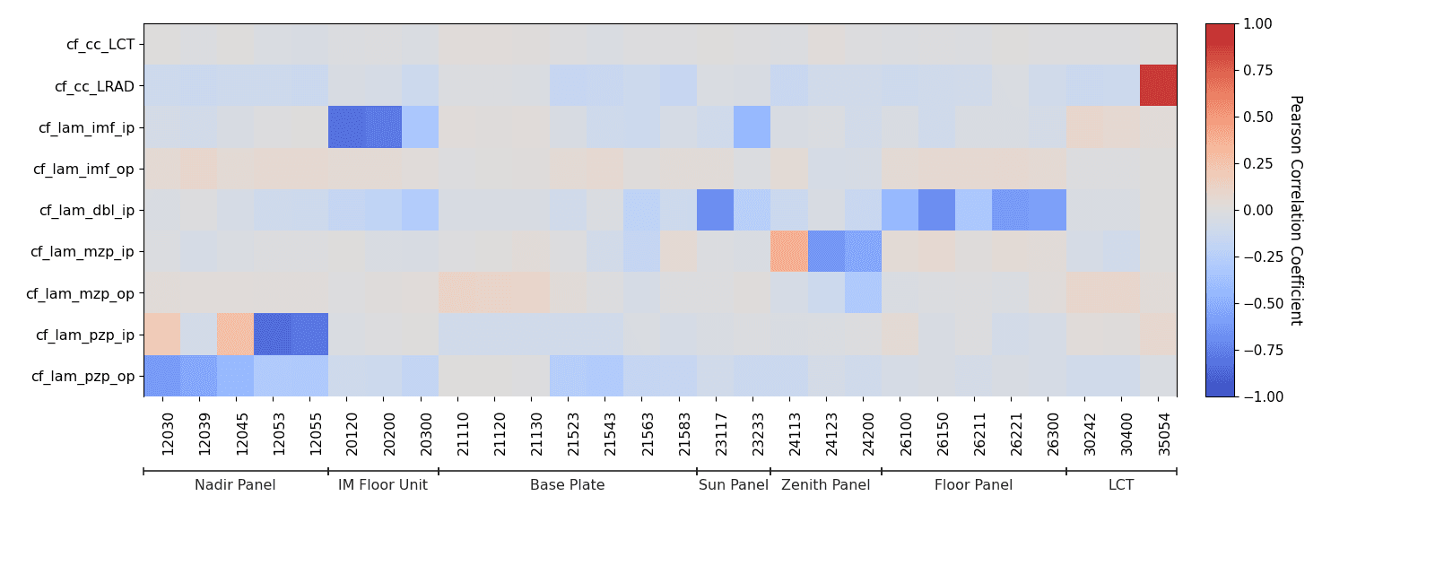
So a sensitivity analysis runs first, ranking parameters by how strongly they move the predicted temperatures at the sensor nodes. It does two jobs at once. Practically, it decides where the sampling budget goes: parameters with negligible influence can be fixed at their nominal values without meaningfully affecting the result. Physically, it is a readable statement about the spacecraft — it names which conductances and couplings actually govern the thermal behaviour of each region, which is useful to a thermal engineer whether or not they ever run a correlation.

The cross-parameter correlation matrix answers the companion question: which parameters are entangled with each other. Strongly correlated pairs cannot be identified independently from this data no matter how long the chain runs, because they trade off to produce the same temperatures — and knowing that in advance stops a converged-looking result from being over-interpreted.

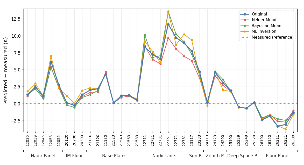
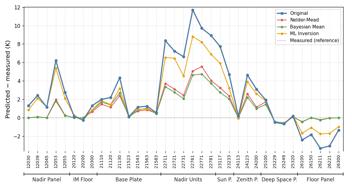
Run against the Sentinel-2 thermal-vacuum data, the pipeline produces a correlated model together with something manual tuning never yields: a quantified statement of how well each parameter is actually known. The final evaluation compares the correlated model's predicted temperatures against the measured sensor data across the test cases — the same check a hand-correlated model is judged on, now reached automatically and reproducibly.

The substantive gain is not that the automated result matches the test better than a careful engineer could manage by hand. It is that the result arrives with its uncertainty attached, is reproducible by someone else from the same inputs, and is explicit about which parameters the campaign identified and which it did not. A correlated model that says 'this conductance is well determined, this one is not' is a more useful input to the next design decision than one that presents every tuned number with equal, unstated confidence.

It also changes what a thermal-vacuum campaign is worth. Because the method reports which parameters the sensor layout actually constrains, it can be turned around and used before a test — to ask where thermocouples should be placed, or which test cases would identify the parameters that matter most.