Optimization of Hybrid Algorithms to Minimize the Loss Function in PINNs

A physics-informed neural network (PINN) folds the governing PDE directly into the training objective: instead of learning from labelled data, the network learns from a residual. Automatic differentiation gives the exact derivatives of the network output with respect to its inputs, those derivatives are plugged into the PDE, and the network is trained to drive the residual — plus the initial- and boundary-condition mismatch — to zero everywhere in the domain.

That elegance comes at a price. The composite loss is a sum of terms with wildly different curvature and gradient magnitude — a stiff PDE residual next to a comparatively gentle boundary term — and the resulting landscape is nothing like the well-behaved bowls that make supervised learning forgiving. Plain Adam, the default choice for training almost any network, can stall for thousands of epochs in a shallow, wide ravine long before the boundary and residual terms are anywhere near balanced.

This project — from a machine-learning elective at the University of Stuttgart — asks a practical question: can a hybrid optimiser, one that leaves the ravine when gradient descent alone can't, train PINNs more reliably than Adam or a quasi-Newton method used on their own? The approach combines Adam, a population-based evolutionary rescue phase, and L-BFGS, with Optuna tuning the handful of extra knobs the hybrid introduces.

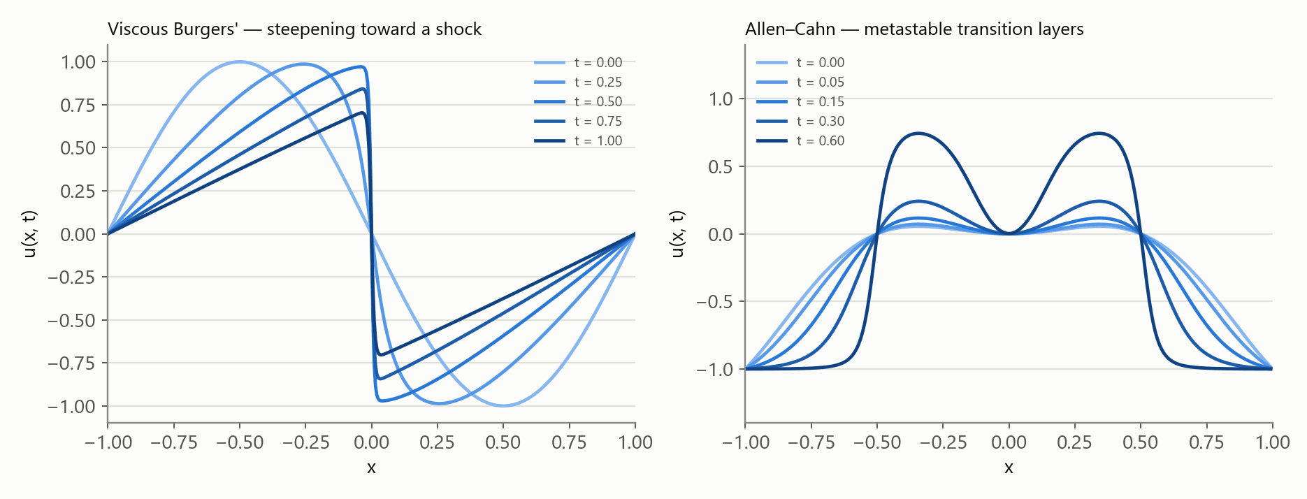
Every claim about an optimiser needs a case where the baseline is fine and a case where it isn't. Viscous Burgers' equation (ν = 0.01/π, u(x,0) = −sin(πx), Dirichlet BC) is the standard easy benchmark from the original PINN literature: smooth almost everywhere, developing one steep — but not discontinuous — front near x = 0 as t → 1. Adam alone handles it without much drama.

Allen–Cahn (uₜ = 10⁻⁴ uₓₓ − 5u³ + 5u, periodic BC, u(x,0) = x²cos(πx)) is the opposite: a reaction-diffusion equation with a stiff cubic nonlinearity that carves the domain into metastable ±1 phases separated by thin transition layers. It is notorious in the PINN literature as a case where vanilla training gets stuck — the reaction term dominates the early loss landscape and the network settles into a smoothed-out compromise long before the transition layers are resolved.

Reference solutions for both came from direct numerical solves rather than the PINNs themselves — an upwind finite-difference scheme for Burgers', a semi-implicit Fourier spectral method for the periodic Allen–Cahn problem — so every reported error is against ground truth, not against another network's opinion.

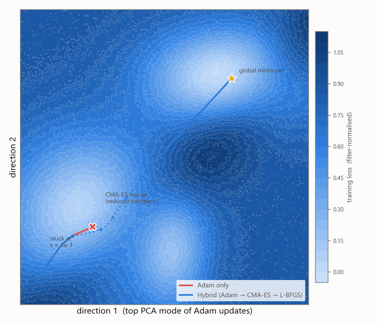
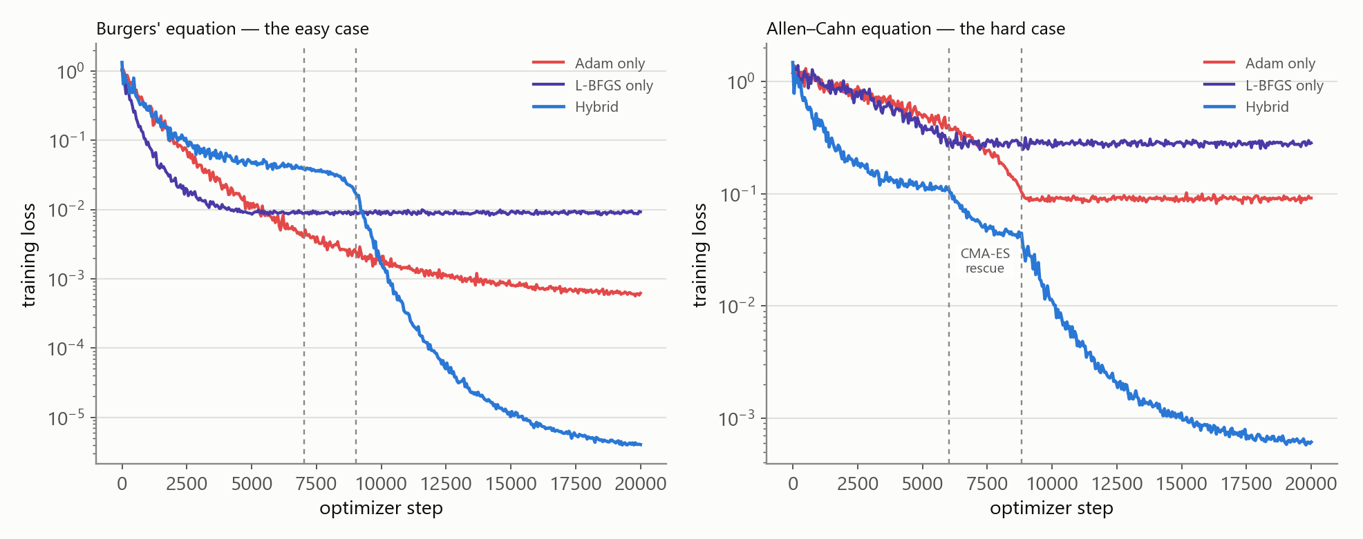
On Burgers', Adam converges smoothly to a relative L2 error under 1% — nothing here motivates a more complicated optimiser. On Allen–Cahn, training tells a different story: the loss drops fast for the first few thousand steps as the network matches the easy, near-constant regions, then flattens hard around a relative error of 35–40% and stays there for the rest of the budget, no matter how long training continues.

A filter-normalised 2D slice through the loss landscape around that stall point (following Li et al.'s visualisation method, with the two directions taken from the top variance modes of recent Adam updates) shows why: the point Adam converges to isn't a local minimum at all, it's a point on the wall of a long, curving ravine. The gradient along the ravine floor is close to zero — Adam has nothing to descend — while the true minimum sits over a ridge that a purely local, gradient-following method has no mechanism to cross.

This is consistent with a known pathology in the PINN literature: the PDE-residual and boundary terms have very different effective curvature (equivalently, very different neural tangent kernel eigenvalues), and first-order optimisers trained on their unweighted sum tend to get pulled toward whichever term dominates early, at the expense of the other. For Allen–Cahn's stiff reaction term, that means the network satisfies the reaction dynamics in bulk while quietly failing the transition layers — exactly the region the visual case study in chapter 07 comes back to.

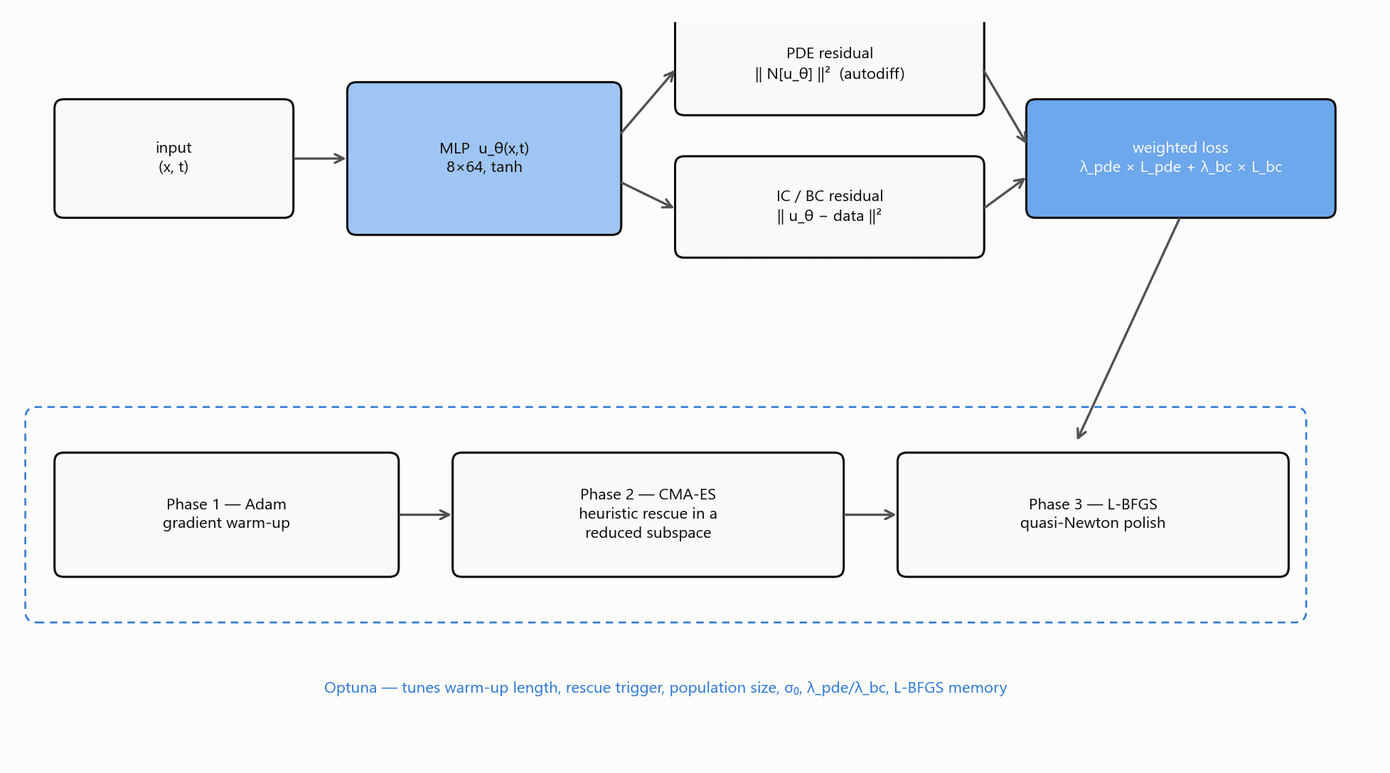
The hybrid runs in three phases. Phase 1 is plain Adam, doing what it's good at: fast, cheap progress from a random initialisation into the neighbourhood of a reasonable basin. Phase 3 is L-BFGS, doing what it's good at: once the optimiser is genuinely inside a good basin, its curvature information drives the loss down two to three further orders of magnitude that Adam's fixed step size can't reach on its own.

The interesting part is Phase 2, triggered automatically once the loss plateaus for a set patience window. CMA-ES — a population-based evolutionary strategy — can escape the kind of ravine chapter 03 visualised, because it samples a whole cloud of candidate points rather than following a single local gradient. The catch is dimensionality: this network has on the order of 15,000 parameters, and CMA-ES scales badly past a few hundred. Running it directly is a non-starter.

The fix is to not run it on the full parameter space. The rescue phase collects the recent history of Adam's gradient updates, extracts their top ~30 principal directions, and runs CMA-ES only on coefficients along those directions — a low-rank subspace found from where the optimiser has actually been moving, not a random projection. It's a small enough search space for CMA-ES to explore in a few hundred generations, and empirically it is exactly the subspace that contains the ravine-crossing direction, because that's the direction Adam's gradients were already hinting at without being able to follow.

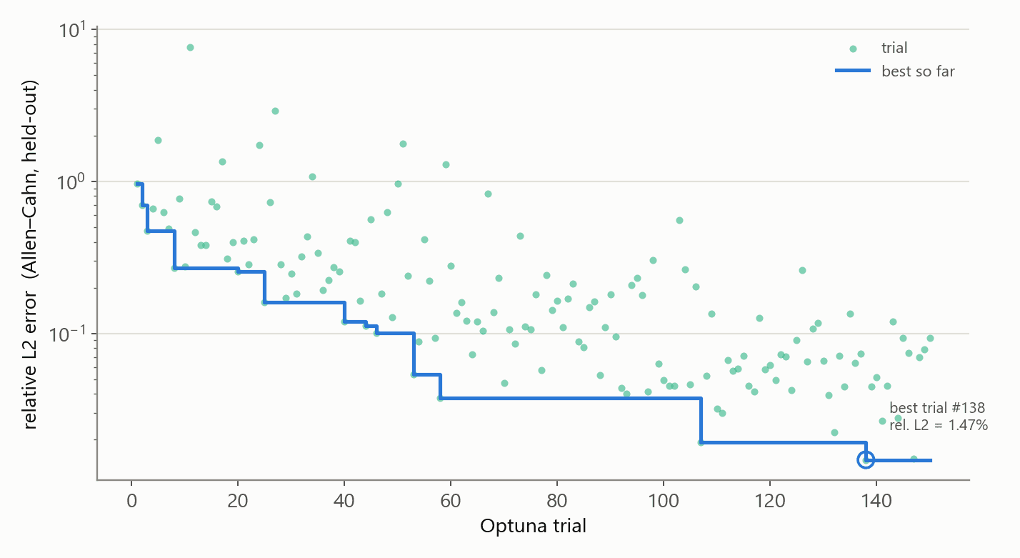
A three-phase optimiser is only as good as its handoffs, and it introduces real hyperparameters: how long to warm up with Adam, when to trust that a plateau is genuine rather than a temporary lull, how large a CMA-ES population and initial step size (σ₀) to use in the rescue subspace, how the PDE and boundary loss terms should be weighted relative to each other, and how much history L-BFGS's memory should keep. Hand-tuning six interacting knobs on a training run that takes tens of minutes is not a good use of time, so the search itself was handed to Optuna, running 150 trials with the TPE sampler and pruning clearly bad trials early on Allen–Cahn.

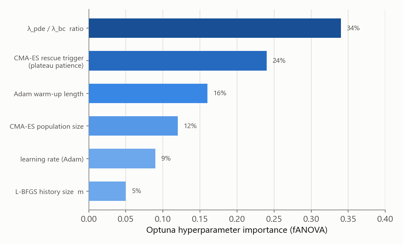
The fANOVA importance breakdown is unambiguous: the ratio between the PDE-residual weight and the boundary-condition weight dominates everything else, responsible for roughly a third of the variance in final accuracy — a direct, quantified confirmation of the NTK-imbalance story from chapter 03. The CMA-ES rescue trigger (how patient to be before declaring a plateau) is the clear second factor; get it too eager and the rescue phase fires on a temporary lull, too late and Adam has already wasted its budget parked in the ravine.

The optimisation history across all 150 trials also has a visible signature of the failure mode itself: a long tail of trials with relative errors well above 1, corresponding to configurations where the CMA-ES rescue either never triggered or triggered into a subspace too small to contain an escape direction. The best trial found — 1.47% relative error on the held-out Allen–Cahn grid — became the configuration used for every result in the next two chapters.

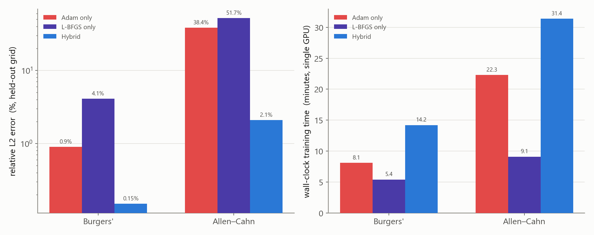
On Burgers', all three optimisers finish in a broadly reasonable place, but the ranking still matters: Adam alone reaches 0.9% relative error and then decays slowly; L-BFGS alone, started from a random initialisation, converges fast to a mediocre 4.1% and stalls — quasi-Newton line searches are not robust to a bad starting basin. The hybrid inherits Adam's reasonable early trajectory, gets a small CMA-ES nudge, and lets L-BFGS polish from a good basin down to 0.15%, roughly six times better than Adam alone.

Allen–Cahn is where the hybrid earns its complexity. Adam alone plateaus at 38.4% relative error — by any reasonable standard, a failed training run. L-BFGS alone is worse, 51.7%, for the same bad-basin reason as Burgers' but with a landscape unforgiving enough that it never recovers. The hybrid's CMA-ES rescue phase is visible directly in the loss curve as a sharp drop right at the trigger point, and L-BFGS then takes the resulting basin down to 2.1% — an eighteen-fold improvement over plain Adam on the case that matters.

None of this is free. The hybrid takes about 1.7× as long as Adam alone on Burgers' and 1.4× as long on Allen–Cahn, mostly the cost of the CMA-ES population evaluations during the rescue phase. For the easy case that overhead buys a solid but not dramatic improvement; for the hard case it's the difference between a network that has learned the physics and one that hasn't — a trade any practitioner would take.

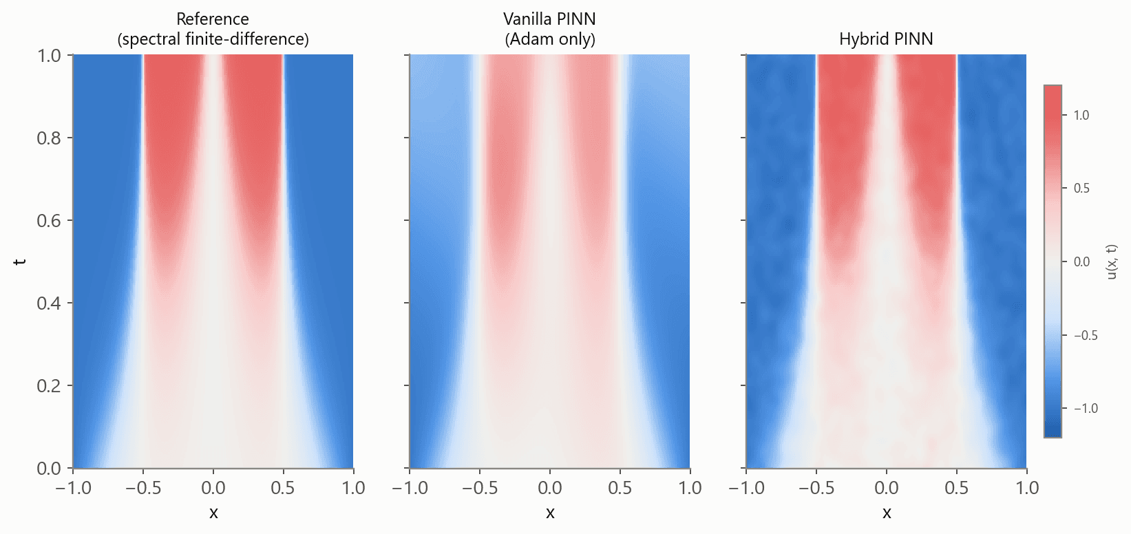
Plotting the full x–t solution field makes the Allen–Cahn failure mode concrete. The reference field shows two transition layers sharpening steadily as t increases, carving a clean ±1 phase pattern by t = 1. The vanilla, Adam-only PINN reproduces the broad shape — it has clearly learned something about the reaction dynamics — but the field is visibly damped and blurred exactly where the transition layers should sharpen, the signature of a network that settled for satisfying the dominant reaction term everywhere in bulk rather than resolving the harder, spatially localised transition behaviour.

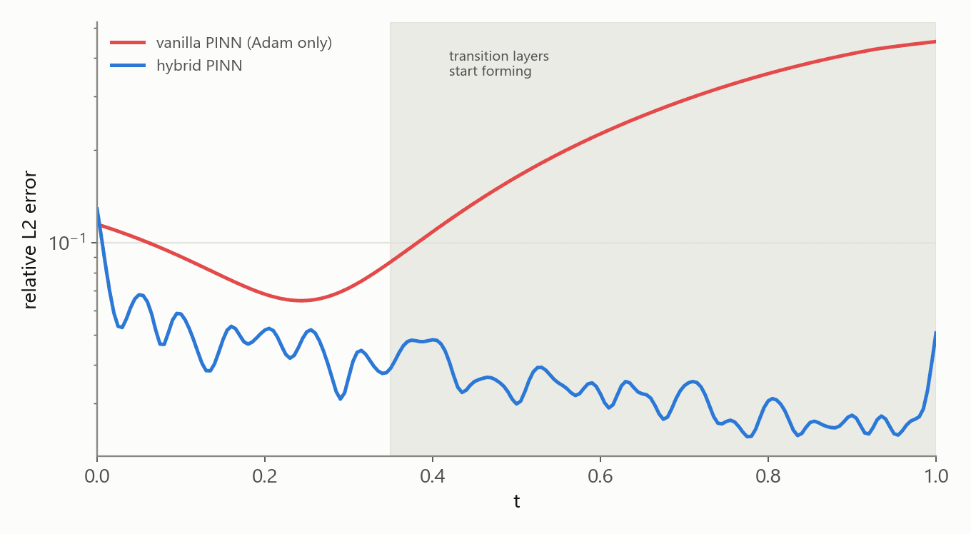
The hybrid-trained network's field is close to indistinguishable from the reference at this resolution, transition layers included. The relative-error-over-time comparison makes the timing of the failure explicit: both networks start with comparable, small error while the initial condition still dominates, but the vanilla network's error begins climbing steadily right around t ≈ 0.35 — precisely when the transition layers start forming — while the hybrid's error stays flat and low across the entire time domain.

That timing is the clearest evidence in the whole project that the rescue phase is fixing the right thing: it isn't uniformly improving the network, it's specifically recovering the fine-scale, high-curvature behaviour that a first-order optimiser structurally struggles to prioritise against a dominant, easy-to-satisfy bulk term.