2D CFD Framework for Interactive Flow Simulation
A from-scratch 2D flow solver with a live, interactive viewer: a vectorized D2Q9 Lattice-Boltzmann core in pure Python/numpy, validated against analytic and benchmark solutions, fast enough to draw obstacles with the mouse and watch a Kármán vortex street form in real time.
A wind tunnel in a window
Every CFD tool I had used at university follows the same rhythm: build a mesh, set up a case, submit, wait, post-process. The feedback loop is measured in hours — which is fine for engineering answers, but terrible for building intuition. What I wanted was the opposite: a small numerical wind tunnel that runs live on a laptop, where you drag a slider and the recirculation bubble grows, where you sketch an obstacle with the mouse and the wake reorganises itself around it within a second.
That goal turns into a hard set of requirements. The solver has to produce a physically credible unsteady flow — not a pretty-but-wrong smoke effect like the classic 'stable fluids' solvers used in games, which are unconditionally stable precisely because they diffuse away the physics. It has to run at interactive rates, tens of solver steps per second, on a mid-range laptop CPU with no GPU. It has to survive whatever geometry a user scribbles into it without a meshing step. And I wanted it in pure Python with numpy as the only numerical dependency — partly as a portability constraint, mostly as a personal challenge: Python is supposedly the wrong language for this.
The result is flowlab, a 2D flow sandbox whose showpiece is the flow every aerodynamicist loves: a cylinder at Re = 150 shedding a Kármán vortex street, computed live — and validated against analytic solutions and published benchmark data, because an interactive toy that gives wrong answers teaches wrong intuition. Every figure and animation on this page is direct output of the framework.
What 'solving the flow' actually means here
The target physics are the incompressible Navier-Stokes equations in two dimensions: conservation of mass (the velocity field stays divergence-free) and conservation of momentum (fluid accelerates under pressure gradients and viscous stresses). Two dimensions is a deliberate, honest reduction — real turbulence is inherently three-dimensional, so this framework is limited to laminar and transitional flows where 2D is a meaningful idealisation: channel flows, bluff-body wakes at moderate Reynolds numbers, cavity flows.
The single number that governs everything is the Reynolds number Re = u·L/ν — the ratio of inertial to viscous forces. At Re below ~5 the flow around a cylinder creeps around it symmetrically; around Re 40 a steady recirculating bubble forms behind it; somewhere near Re 47 that bubble becomes unstable and starts shedding vortices periodically. A solver that is interactive across that range lets you watch these bifurcations happen — which was the entire point of the project.
Interactivity also dictates the numerical priorities, and they differ from classical CFD. Per-step accuracy matters less than robustness (a user will absolutely draw an obstacle straight into the inflow), memory locality matters more than formal convergence order, and everything must vectorise — in Python, any per-cell loop is death: a single interpreted loop over a 720×240 grid costs more than an entire vectorised solver step.
Attempt one: a classical projection solver
The first implementation was the textbook route: Chorin's projection method on a staggered marker-and-cell grid. Advance the momentum equation explicitly to get a provisional velocity field, then project it back onto the space of divergence-free fields by solving a Poisson equation for pressure, whose gradient corrects the velocity. Semi-Lagrangian advection kept the time step stable; central differences handled diffusion. It worked — and it taught me exactly why interactive CFD is hard.
The Poisson solve is the killer. It is a global elliptic problem: information from every cell must propagate to every other cell within a single time step, because in an incompressible fluid pressure acts instantaneously. With Jacobi or Gauss-Seidel iterations, driving the divergence residual down properly on a 720×240 grid took several hundred iterations per step — two orders of magnitude more work than the rest of the step combined. Truncating at 40–60 iterations, as real-time smoke solvers do, leaves residual divergence: mass quietly appears and disappears near the obstacle, drag values drift, and the wake frequency depends on the iteration cap. FFT-based Poisson solvers are fast but demand periodic or simple box boundaries — incompatible with mouse-drawn obstacles.
I spent a while fighting this with better solvers (red-black SOR, a rough multigrid) before accepting the structural conclusion: the projection method's global coupling is fundamentally at odds with both interactivity and numpy's array-at-a-time execution model. What I needed was a scheme where every operation is local. That scheme exists, and it comes from an unexpected direction — statistical mechanics.
Lattice-Boltzmann: solving Navier-Stokes without ever seeing it
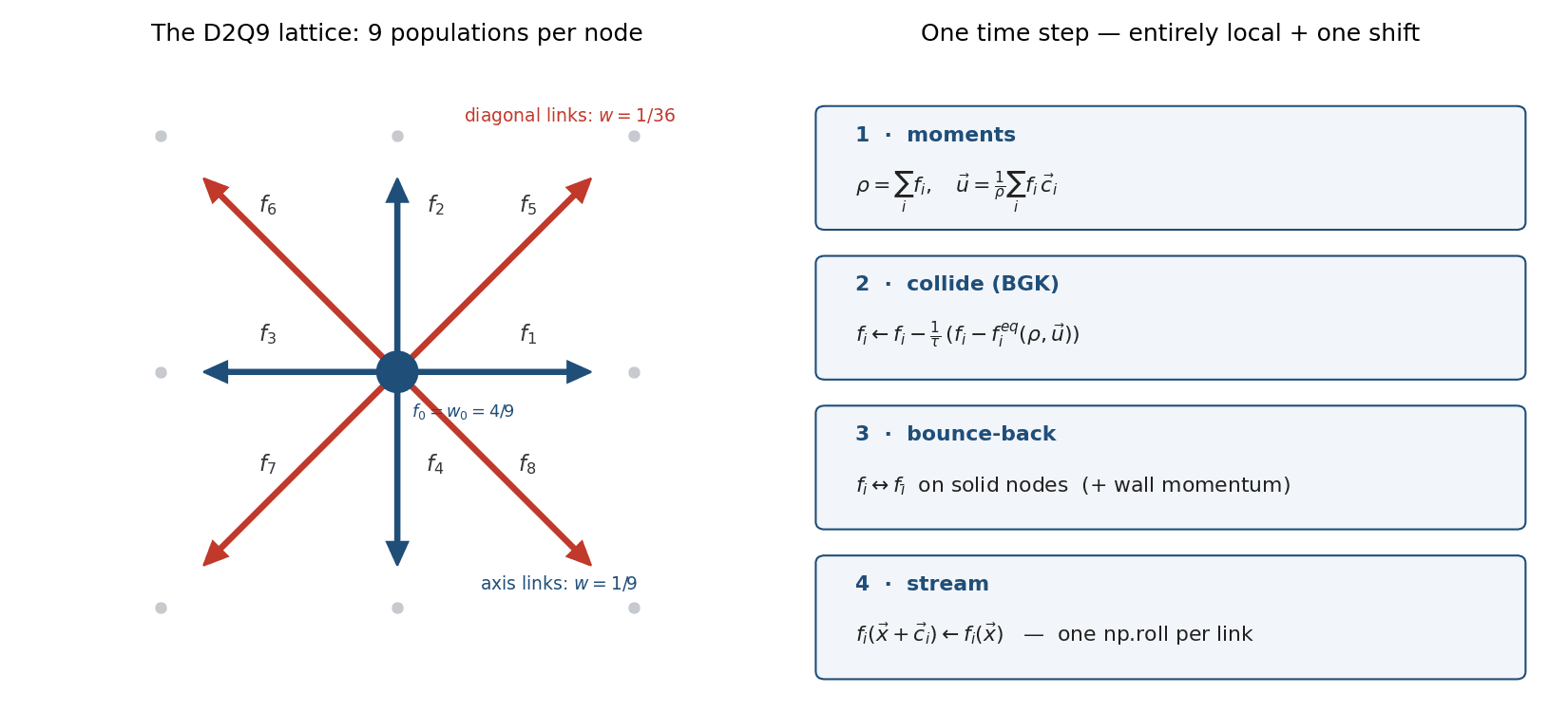
The Lattice-Boltzmann method doesn't discretise the Navier-Stokes equations at all. It simulates a heavily stylised gas: at every grid node live nine particle populations f₀…f₈ (the D2Q9 lattice), each representing the mass travelling with one of nine discrete velocities — rest, the four axis directions, and the four diagonals. Each time step does two things. Collide: at every node, the populations relax toward a local Maxwell-Boltzmann-like equilibrium computed from the node's density and velocity. Stream: every population hops one lattice link in its travel direction.
The magic is that this microscopic caricature has the right macroscopic limit: a Chapman-Enskog expansion shows that density and momentum moments of the populations obey the incompressible Navier-Stokes equations to second order, with the kinematic viscosity set by the relaxation time τ of the collision step, ν = (τ − ½)/3 in lattice units. Pressure — the expensive global unknown of the projection method — becomes a local quantity, just ρ/3: the model behaves like a very-low-Mach compressible gas in which pressure waves carry the incompressibility information at finite speed instead of infinitely fast.
For this project the trade is perfect. Both steps are completely local: collision is pure per-node arithmetic, streaming is a fixed shift of nine arrays — numpy's roll(). No iteration, no linear system, no convergence check, no mesh. Geometry is a boolean mask. The BGK single-relaxation-time collision operator — the simplest closure, with all its documented weaknesses at high Reynolds numbers — was chosen deliberately: this framework lives at laminar Re where BGK is accurate, and its simplicity is what keeps the inner loop at interactive speed.
The whole solver is ~120 lines of numpy
The state of the simulation is a single float32 array of shape (9, Ny, Nx) — nine population fields. One time step: sum the populations for density; take their first moments for momentum; build the equilibrium distribution feq = w·ρ·(1 + 3(c·u) + 4.5(c·u)² − 1.5u²) for all nine directions at once via broadcasting; relax f toward it with f += (feq − f)/τ; then stream each direction with one np.roll per link. Every line is an array operation over the full grid — there is not a single Python loop over cells anywhere in the solver.
Two implementation choices bought most of the speed. First, float32 instead of float64 halves memory traffic — and LBM on a modern CPU is memory-bandwidth-bound, not compute-bound, so this is nearly a factor-two speedup for free at laminar accuracy levels (with one caveat the validation chapter will confess to). Second, moments are computed as explicit signed sums of the nine arrays rather than generic tensor contractions, which keeps everything in flat, cache-friendly passes.
The equations of the collision step never mention Navier-Stokes, pressure or viscosity — yet drag forces, boundary layers and vortex streets fall out of the moments. There is something genuinely delightful about a solver whose inner loop would fit on a slide, and I kept it that way on purpose: no operator classes, no plugin registry, no premature architecture. A solver core you can read top to bottom in five minutes is a feature, not a lack of ambition.
Walls that are just pixels
Solid geometry in this framework is a boolean mask over the grid — true means wall. The physics at walls is handled by bounce-back: populations that stream into a solid node are reversed and sent back where they came from next step. That single rule enforces no-slip, works for any pixelated shape with no meshing, no normals and no special cases, and is exactly what makes mouse-drawn obstacles trivial: the brush just sets mask pixels, and the solver picks them up on the next step. The mask trick has one classic subtlety — the effective wall sits half a lattice link inside the fluid, which the validation cases have to account for.
Moving walls get one extra term: the lid of the driven-cavity case adds momentum 6wᵢρ(cᵢ·u_wall) to each reflected population — the standard moving-wall bounce-back correction. The domain inlet imposes an equilibrium distribution at the prescribed inflow velocity on the left column; the outlet is a zero-gradient copy of the second-to-last column, which lets vortices leave with only mild reflections. These first-order boundary treatments are the crudest part of the framework, and I list them as such under limitations — but they are robust against everything a user can draw, which for a sandbox outranks formal order.
Bounce-back also hands over aerodynamic forces almost for free, via momentum exchange: every population reversed at an obstacle transfers momentum 2cᵢfᵢ to it, so summing that over all boundary links each step gives the instantaneous drag and lift vector on the body — no pressure integration, no surface reconstruction. That one summation turns the sandbox into a measuring instrument, and chapter 11 hangs actual numbers on it.
The bookkeeping that makes it physics
LBM computes in its own units: grid spacing 1, time step 1, reference density 1. Nothing in the solver knows about metres or seconds — physical meaning is imposed afterwards by matching dimensionless numbers. For a cylinder of D lattice nodes in an inflow of u₀ lattice units per step, the viscosity that realises a target Reynolds number is ν = u₀·D/Re, which fixes the relaxation time τ = 3ν + ½. Match Re, and every dimensionless output — Strouhal number, drag coefficient, normalised velocity profiles — is directly comparable to experiments.
The free parameters live inside hard stability fences. The lattice Mach number u₀/cₛ (with cₛ = 1/√3 the lattice sound speed) must stay small, since LBM is a weakly compressible model of an incompressible flow — I run u₀ = 0.1, giving Ma ≈ 0.17 and density fluctuations well under one percent. And τ must stay safely above its stability limit of ½: as τ → ½ the BGK collision loses dissipation and the simulation blows up in a checkerboard of noise. The Re = 150 cylinder runs at τ ≈ 0.556 — comfortable; pushing the same grid toward Re ≈ 1000 would drive τ ≈ 0.508, which is where BGK starts to live dangerously.
Those two fences together define the framework's envelope: at fixed resolution, Reynolds number can only be raised so far before either compressibility errors or collision instability bite. Higher Re honestly requires more nodes across the obstacle — the interactive version therefore exposes Re only within a per-resolution safe range, computed from these constraints, rather than letting the user discover the stability boundary by detonation.
Poiseuille flow: the solver meets an exact solution
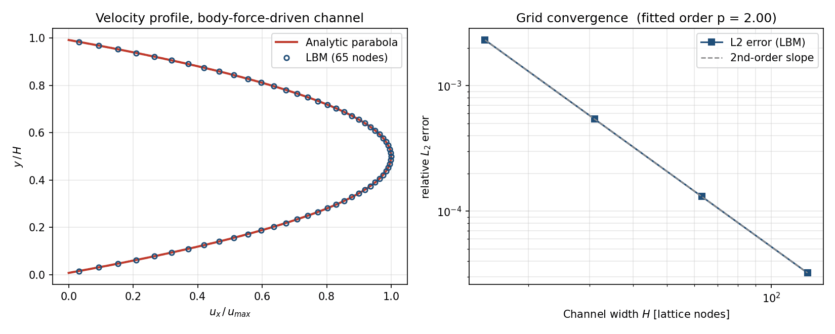
Validation started with the one flow where the answer is exact: body-force-driven channel flow, whose steady profile is the textbook parabola u(y) = g·y(H−y)/2ν. The simulated profile lies on the analytic curve to within a fraction of a percent — and the first thing this case caught was not an error in the solver but in my analysis: the L2 error initially converged at first order, which turned out to be the half-link wall offset of bounce-back. The effective channel width is Ny − 2, not Ny − 1; fitting a parabola through the computed profile put the no-slip planes at y = 0.504 and y = 31.496 — half a link inside the fluid, exactly as the theory says.
With the wall position corrected, the grid refinement study gives a fitted convergence order of p = 2.00 across channel widths of 15 to 127 nodes — the second-order accuracy LBM promises. Getting that clean slope required a second, more embarrassing fix: in float32, the finest grid refused to converge below ~0.2% error. The per-step body force there is ~2×10⁻⁶ — six orders of magnitude below the populations it increments, right at single-precision resolution, so round-off noise floored the study. The production solver stays float32 for speed; the convergence study runs in float64. A tidy lesson in how 'performance settings' and 'validation settings' are not the same thing.
The final numbers: relative L2 profile errors of 0.23%, 0.054%, 0.013% and 0.0032% for 15, 31, 63 and 127 nodes across the channel. For a method whose wall is literally a row of boolean pixels, that is a satisfying place to start from.
The lid-driven cavity vs. forty years of benchmark data
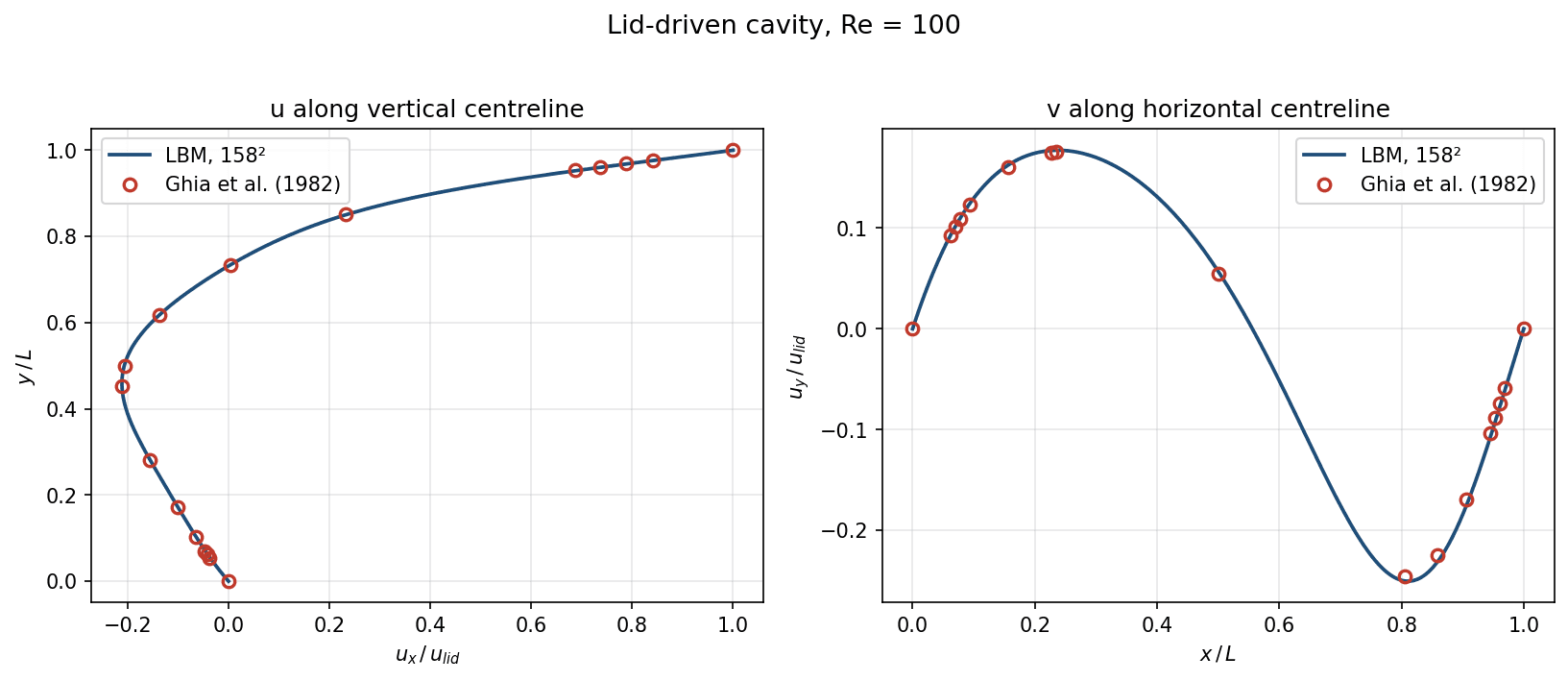
The lid-driven cavity is CFD's drosophila: a square box, three fixed walls, a lid sliding at constant speed — deceptively simple, no analytic solution, and benchmarked to death since Ghia, Ghia & Shin published their reference solutions in 1982. Every CFD code is expected to reproduce their centreline velocity profiles, so this framework had to as well: Re = 100 on a 158² fluid grid, moving-wall bounce-back on the lid, run to steady state.
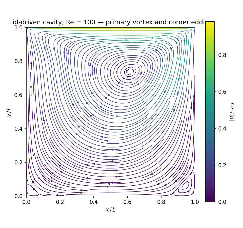
The computed u-velocity along the vertical centreline and v-velocity along the horizontal centreline sit on Ghia's seventeen tabulated points with RMS deviations of 0.22% and 0.32% of lid speed respectively — comfortably within what the 1982 reference itself resolves. The streamline picture shows the right topology too: primary vortex slightly off-centre toward the lid's driving direction, and the two counter-rotating corner eddies at the bottom, small enough that they only appear once the streamline seeding is dense.
This case stresses entirely different code paths than the channel: the moving-wall momentum term, corner nodes where two walls meet, and long transients (the flow needs on the order of a hundred thousand steps to truly settle at this size — steady-state work is where interactive-first design pays nothing). Passing both validations with the same unmodified core is what let me trust everything the sandbox shows from here on.
A Kármán vortex street, live
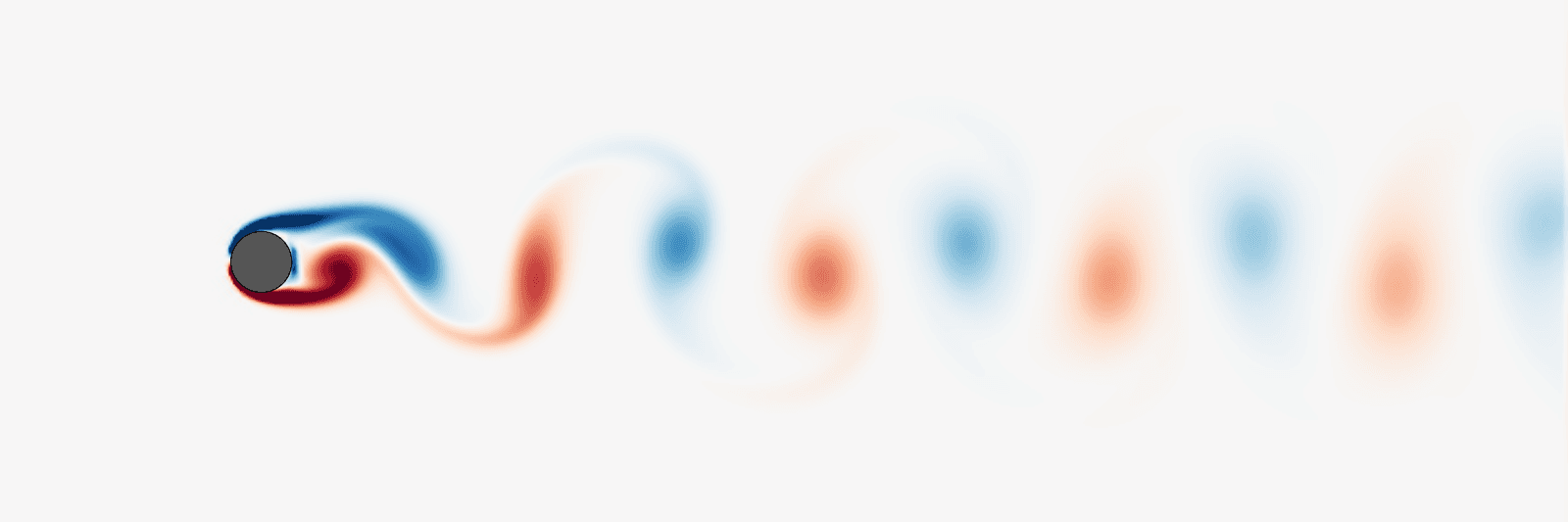
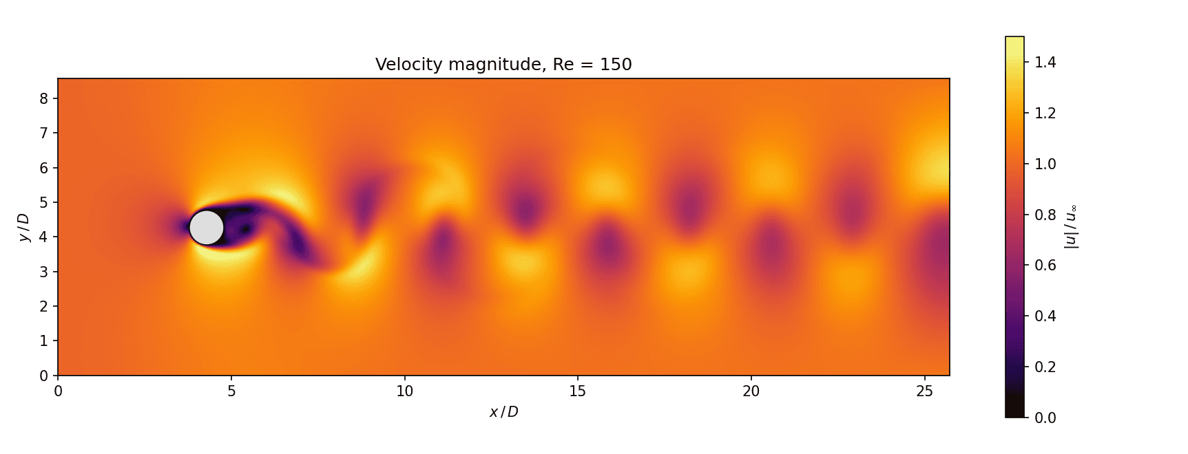
With the physics trusted, the flow the whole project was built for: a circular cylinder of 28 lattice nodes diameter in a 720×240 channel at Re = 150 — squarely in the regime where the wake is periodically unstable. The steady twin-vortex solution exists but is unstable; any asymmetry grows, the recirculation bubble starts to wobble, and the flow settles into the celebrated vortex street: vortices of alternating sign peeling off the upper and lower shoulders and riding downstream in two staggered rows.
The animations show the developed street computed by the framework — vorticity in red-blue (each red vortex spins counter-clockwise, each blue one clockwise) and velocity magnitude in heat colours, where the wake meanders like a flag between the passing vortices. In the interactive viewer this is the default scene, and it is genuinely mesmerising to perturb: nudge the Reynolds slider down below ~47 and the street heals into a steady bubble; nudge it back up and the instability re-grows over a few hundred steps, exactly as the stability theory says it should.
A practical note on honesty in these animations: the simulation is seeded with a small transverse velocity perturbation downstream of the cylinder so the instability saturates after ~15 shedding periods instead of ~50. Without the seed the same street develops from accumulated round-off asymmetry alone — it just takes several times longer to arrive. Physics doesn't need the help; my patience did.
Strouhal number and forces: the street quantified
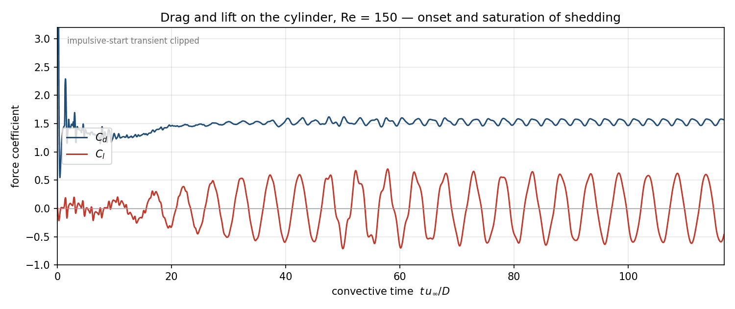
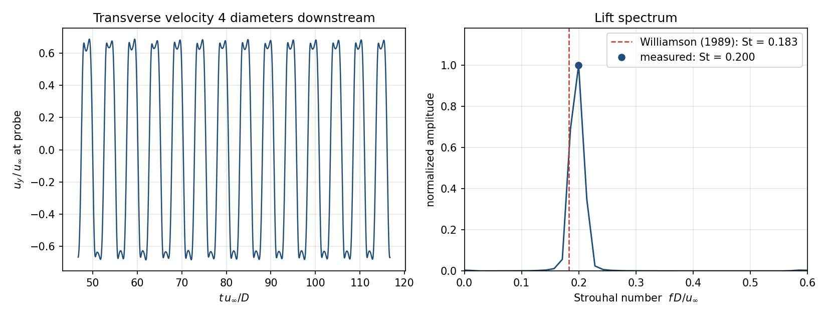
A vortex street that merely looks right proves nothing — bluff-body wakes have been measured for a century, so the framework's street has to hit known numbers. The momentum-exchange summation from chapter 06 records drag and lift every ten steps, and the force history tells the whole life story of the flow: drag settles first while the wake is still symmetric and lift hovers near zero; then the instability grows, lift begins to oscillate with exponentially increasing amplitude, and the flow locks into its limit cycle — with drag oscillating at exactly twice the lift frequency, since each of the two vortices per cycle gives one drag kick.
The shedding frequency is the classic scorecard. A Hann-windowed FFT of the saturated lift signal puts the dimensionless shedding frequency at St = f·D/u∞ = 0.200, against Williamson's unconfined experimental value of 0.183 for Re = 150 — 9% high, and that offset is not noise but physics: the domain confines the cylinder with 12% blockage, the bypassing flow accelerates, and confined-cylinder studies report exactly this upward shift in St. The time-averaged drag lands at Cd ≈ 1.53 with a lift amplitude of ±0.70, against ≈ 1.33 and ≈ 0.5 for an unconfined smooth cylinder — again elevated in the direction and rough magnitude the blockage plus the staircase surface predict. Chasing those residuals to their known causes, rather than tuning until the headline number matched, was a deliberate choice: the framework should report what its assumptions imply, visibly.
These probes are cheap enough to leave running permanently, so the interactive viewer displays live Cd, Cl and a running Strouhal estimate while you play — which quietly turns 'watch the pretty vortices' into 'watch Cd jump when you make the obstacle blunter', and that is exactly the intuition-building the project was for.
Re = 40 vs. Re = 150: the bifurcation on screen
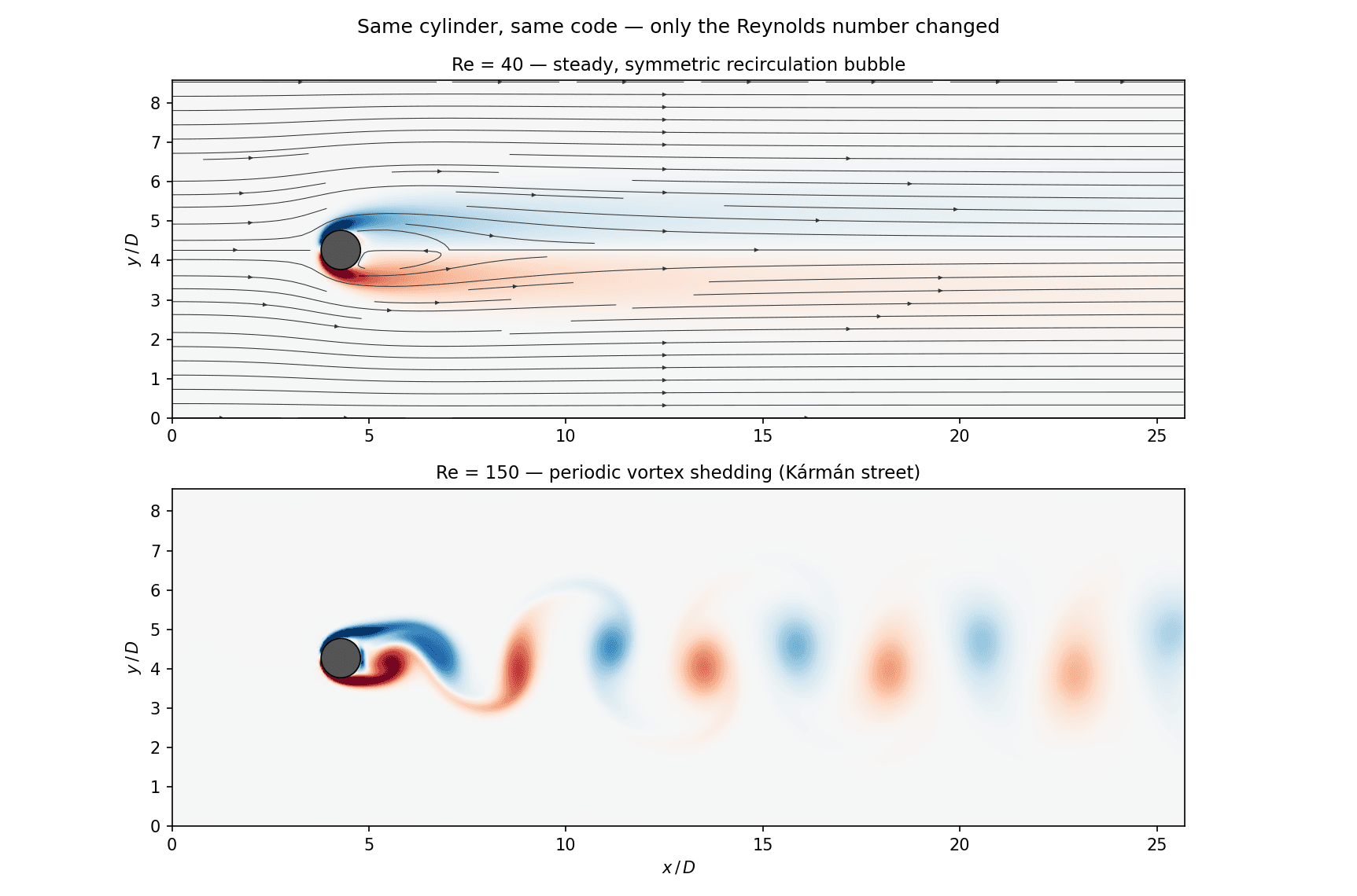
The most instructive experiment the sandbox offers costs one slider movement. At Re = 40 the wake is a steady, mirror-symmetric pair of counter-rotating recirculation bubbles about two diameters long — the flow field converges and then simply stops changing. At Re = 150, with identical geometry, grid and code, no steady solution is reachable at all: the symmetric state is linearly unstable, and the flow inevitably finds the periodic street.
Between them, near Re ≈ 47, sits a genuine supercritical Hopf bifurcation — one of the cleanest examples in fluid mechanics of a system trading a fixed point for a limit cycle as a parameter crosses a threshold. Watching the transition live, both directions, does more for intuition about flow stability than any number of lecture slides did for me; it is the single feature of the framework I'd defend hardest.
Sliders, brushes and arbitrary geometry
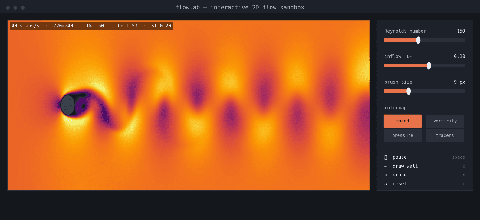
The viewer wraps the solver in an event loop that renders every few solver steps into a live field view — speed, vorticity, pressure (ρ/3), or passive tracer particles advected with the flow. Parameters bind to sliders: inflow velocity applies instantly at the inlet; the Reynolds slider recomputes τ on the fly, clamped to the stability envelope from chapter 07 so no slider position can crash the physics. Everything renders through the same double-buffered numpy-to-bitmap path, and the field data is the solver's actual state — there is no separate 'display simulation'.
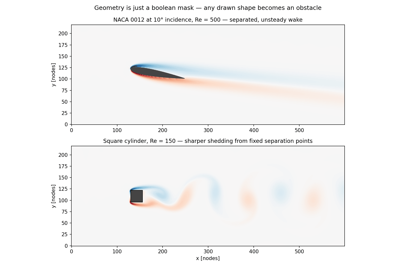
Geometry is where the mask representation earns its keep: a brush sets or clears solid pixels while the simulation runs, so you can build a splitter plate behind the cylinder mid-shedding and watch the street stabilise — a classic flow-control experiment from the literature, reproduced by doodling. The gallery shows the range: a NACA 0012 airfoil at 10° incidence with a separated, unsteady suction-side wake at Re = 500, and a square cylinder whose fixed separation corners produce a harder-edged street than the round one. Both are just different boolean masks fed to the identical core.
One engineering subtlety: freshly drawn solid cells simply adopt bounce-back behaviour with whatever populations they contained, and erased cells re-enter the fluid initialised at local equilibrium. Both operations inject a small, localised disturbance — physically dubious for one time step, gone within a few dozen. A cleaner refill scheme (interpolating populations from fluid neighbours) is on the roadmap; in practice the artefact is invisible next to the disturbance the new geometry itself causes.
How fast can numpy pretend to be a gas?
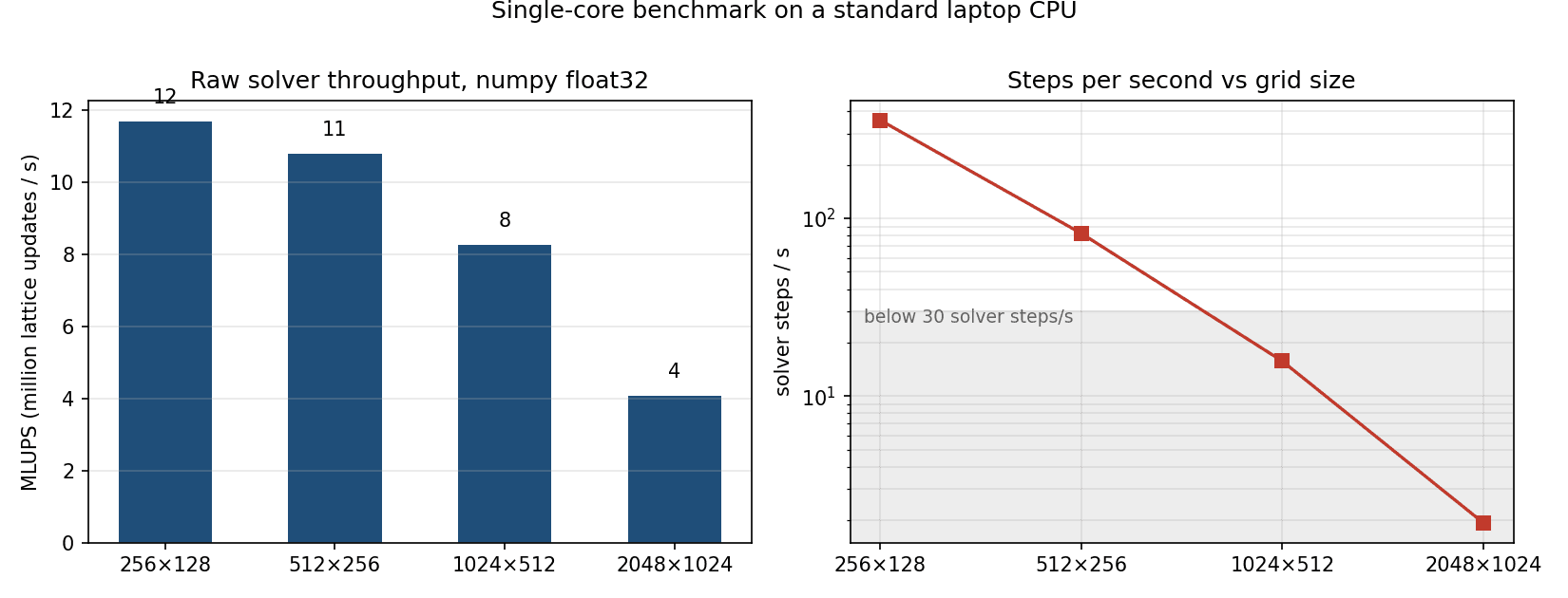
The honest metric for LBM throughput is MLUPS — million lattice-site updates per second. Benchmarked single-core on a standard laptop CPU, the solver sustains 4–12 MLUPS depending on grid size, with the sweet spot at mid-sized grids: small grids drown in per-call numpy overhead (dozens of array operations per step, each with fixed cost), while the largest grids spill out of the last-level cache and become pure memory-bandwidth exercises.
In frame-rate terms: the 720×240 showcase grid runs at ~45 solver steps per second, and since smooth perception needs only ~25 rendered frames per second with a handful of solver steps in between, that is comfortably real-time. A 1024×512 grid — half a million cells — still turns over several steps per second: usable for a 'fast-forward' rather than live mode. For pure Python with one dependency, I consider that the thesis proven: the language was never the bottleneck, the algorithm choice was.
The measured numbers also chart the road not yet taken: the same algorithm ports almost mechanically to GPU (every operation is a map or a shift — LBM is famously the friendliest CFD algorithm to accelerators), and published GPU implementations reach thousands of MLUPS. A CuPy backend — swapping the array module, nothing else — is the single highest-leverage item on the roadmap.
What this framework is not
Every result on this page lives inside explicit assumptions, and listing them is part of the engineering. Dimensionality: strictly 2D — above Re ≈ 190 a real cylinder wake develops three-dimensional instabilities, so 2D results beyond that are a mathematical idealisation, not a prediction. Regime: laminar only — BGK with no turbulence model; wall resolution and collision stability cap the practical envelope around Re ≈ 10³ at sandbox resolutions. Compressibility: LBM is weakly compressible — results carry O(Ma²) ≈ 1–3% error at the u₀ = 0.1 operating point, visible as faint acoustic waves bouncing through the domain after abrupt changes.
Boundaries are first-order: bounce-back renders every surface as a pixel staircase whose effective position sits half a link into the fluid — fine for a 28-pixel cylinder, genuinely distorting for a thin airfoil trailing edge. The zero-gradient outlet reflects a small fraction of each departing vortex; the domain (26 diameters long, 12% blockage) confines the flow, which is worth 9% on the Strouhal number and ~15% on drag versus unconfined references — quantified in chapter 11, not hidden. Collision: single-relaxation-time BGK ties the bulk viscosity to the shear viscosity and loses accuracy as τ → ½; a TRT/MRT operator would decouple these at ~30% more cost. Precision: float32 throughout — validated as sufficient for the flows shown, but demonstrably (chapter 08) not for fine-grid convergence studies.
None of these are apologies — they are the price of the design goals, paid consciously. A framework that admits exactly where it stops being trustworthy is more useful, and frankly more employable as an engineering exercise, than one that claims generality it can't validate. The one-line summary: quantitatively credible laminar 2D flows at interactive speed — nothing more, and demonstrably nothing less.
What building it taught me
The loudest lesson is algorithmic: when a method fights your execution model, change the method, not the language. Attempt one failed not because Python is slow but because the projection method's global pressure coupling multiplies whatever per-operation cost exists; LBM's locality made the same hardware feel two orders of magnitude faster. Second, validation has its own failure modes: of the three initially 'wrong' results in this project, zero were solver bugs — one was a mis-specified effective wall position, one was float32 round-off in the error metric, one was an unconverged transient polluting a convergence study. The solver was right; the measurements weren't. That inverted debugging instinct — suspect the ruler before the physics — is the most transferable thing I took from this.
And it connects forward: the moment interactive flow becomes cheap, it stops being a demo and becomes an instrument. I have used the sandbox to sanity-check separation behaviour before setting up 'real' RANS cases, and to explain vortex shedding to non-engineers in about ninety seconds, mouse in hand.
The roadmap, in order of leverage: a CuPy/GPU backend (same code, thousand-fold headroom); a TRT collision operator plus interpolated bounce-back to push accuracy at higher Re; a Smagorinsky-type subgrid model as an honest, clearly-labelled way to let the sandbox gesture at turbulent regimes; and passive scalar transport for live heat-plume demos. Each slots into the same ~120-line core — which is, in the end, the strongest argument for having kept it small.