Structural Analysis of a Bridge Under Various Load Cases

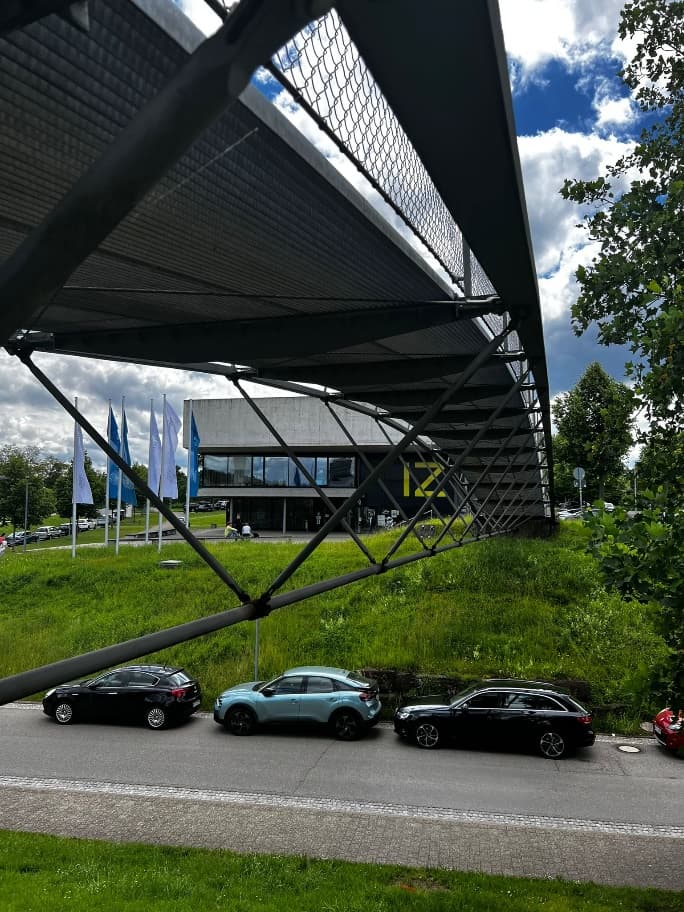
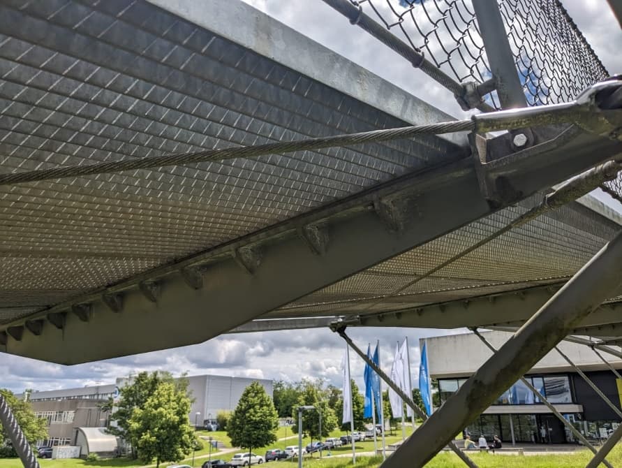
For the applied finite-elements seminar at the University of Stuttgart, our four-person team got a real structure instead of a textbook cantilever: a slender steel arch footbridge — two arches carrying the walkway on twelve cross-girders, each braced by V-struts, the whole deck stiffened by X-tension cables under pre-tension. Total structural mass: about 15 tonnes of steel for a full pedestrian span, which is remarkably light — and, as it turned out, the single most important fact about its dynamics.

The bridge was documented in an architecture journal when it was built (Detail 12/1999), including one number that would become our benchmark long before we ran any experiment of our own: a measured natural frequency of about 2.1 Hz.

The brief for the semester: build the model from geometry up — mesh, convergence study, modal analysis, damping — then subject it to realistic dynamic load cases and, finally, check the simulation against reality. The whole journey, from CAD to jumping on the actual bridge with an accelerometer, is documented below.

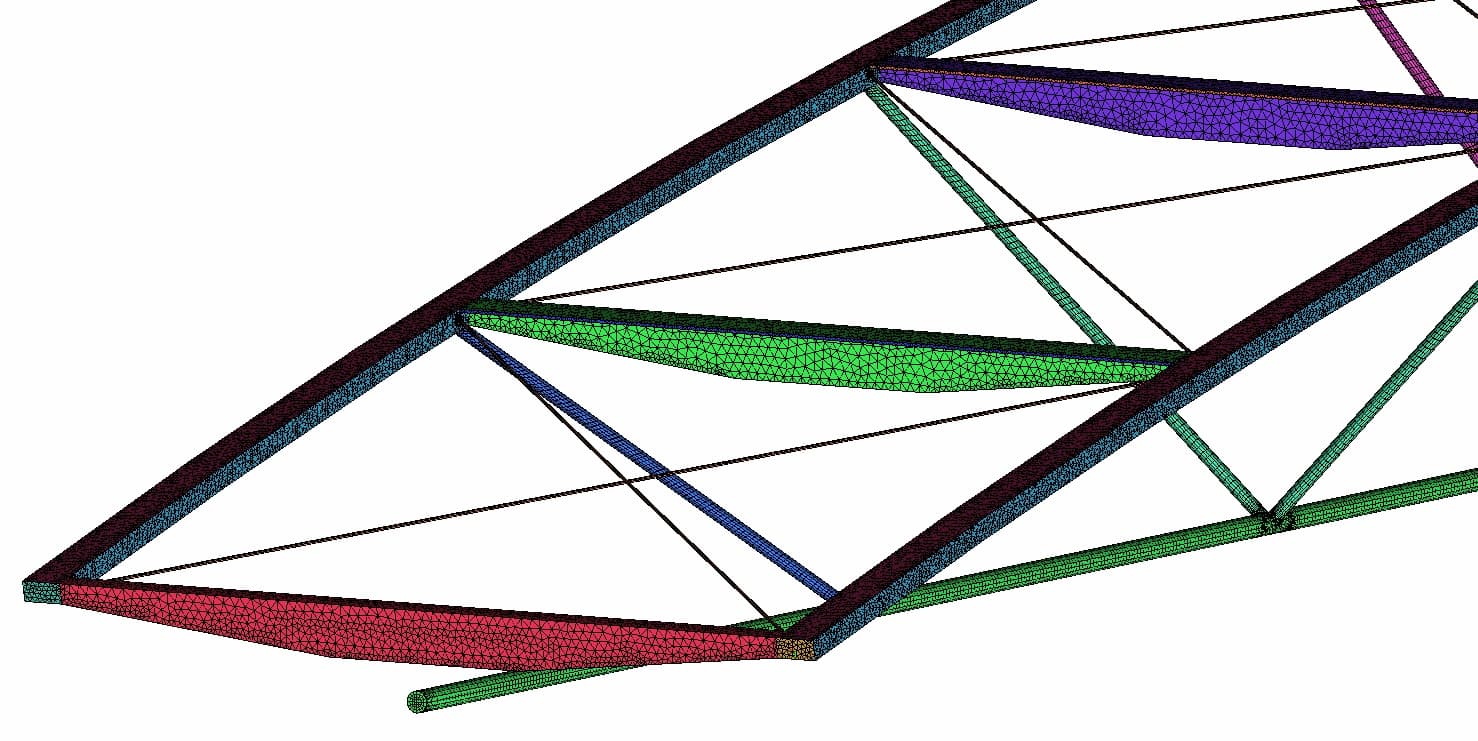
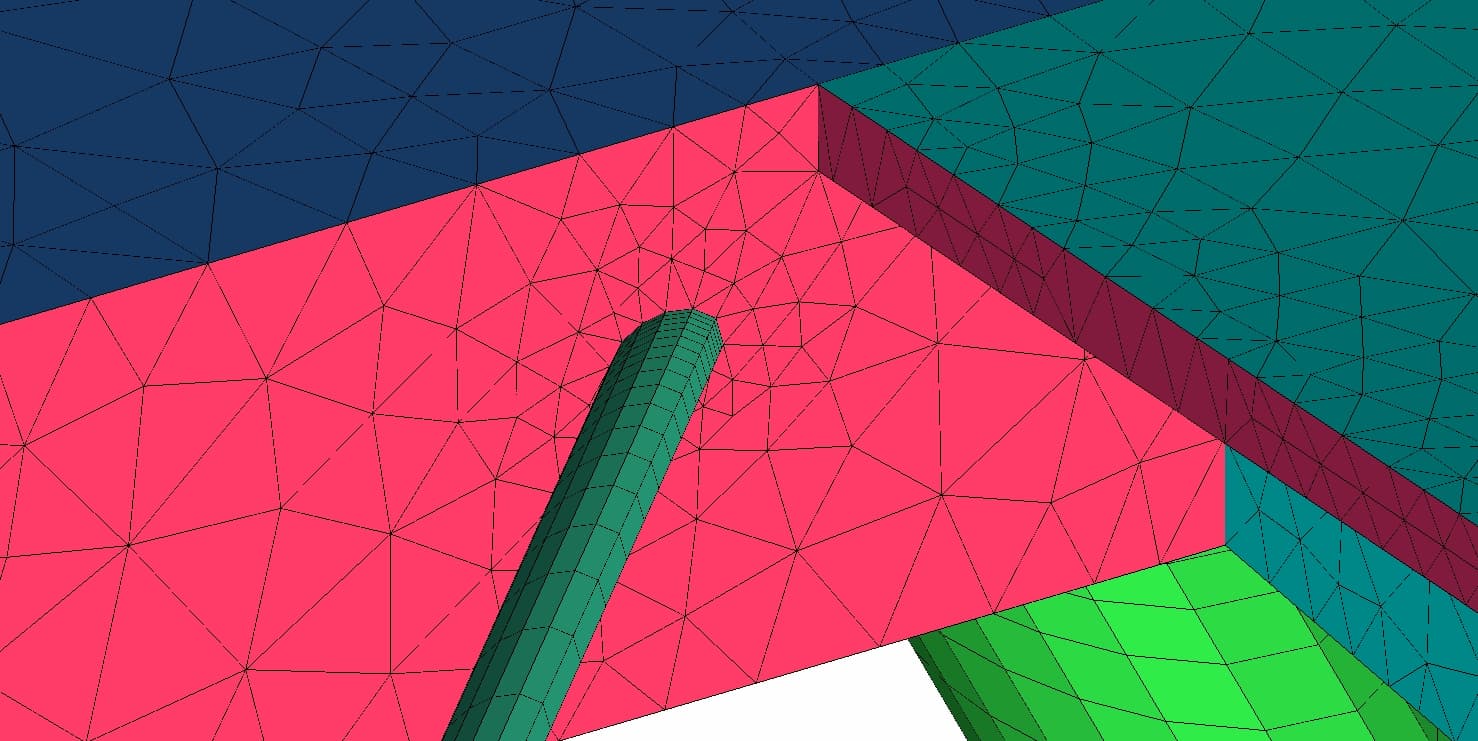
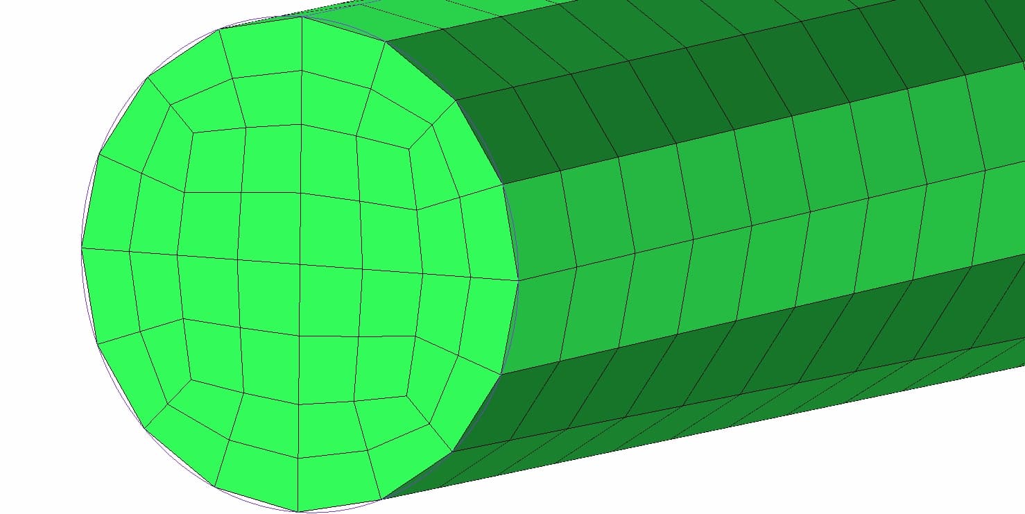
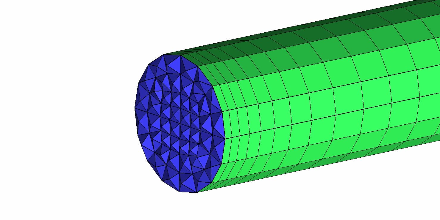
The mesh was built in ANSYS ICEM R21.2 as a deliberate hybrid, with quadratic shape functions throughout. The geometrically messy parts — arches and cross-girders — got unstructured tetrahedra from the Octree/Delaunay mesher, with local size prescriptions steering the resolution: 75 mm on the arches, 30 mm on cross-girders, down to 10 mm along girder edges and 5 mm at the cable interfaces. The slender circular members — X-cables, V-struts and the longitudinal cable — were meshed as structured hexahedra instead: a blocking with prescribed node distributions, and O-grids to discretise the round cross-sections cleanly.

Tet and hex meshes cannot be joined conformally, so every transition got a layer of pyramid elements — small interfaces that keep the mesh watertight where a V-strut meets the longitudinal cable or a cable lands on a girder.

The part that saved us weeks: ICEM is fully scriptable in TCL. Cell sizes, blocking node distributions and growth ratios all live in variables and loops instead of dialog boxes, so the entire mesh is parametrised — change one size parameter and the whole bridge remeshes consistently, with size ratios preserved independently of the absolute cell size. That one property is what made the convergence study practical.

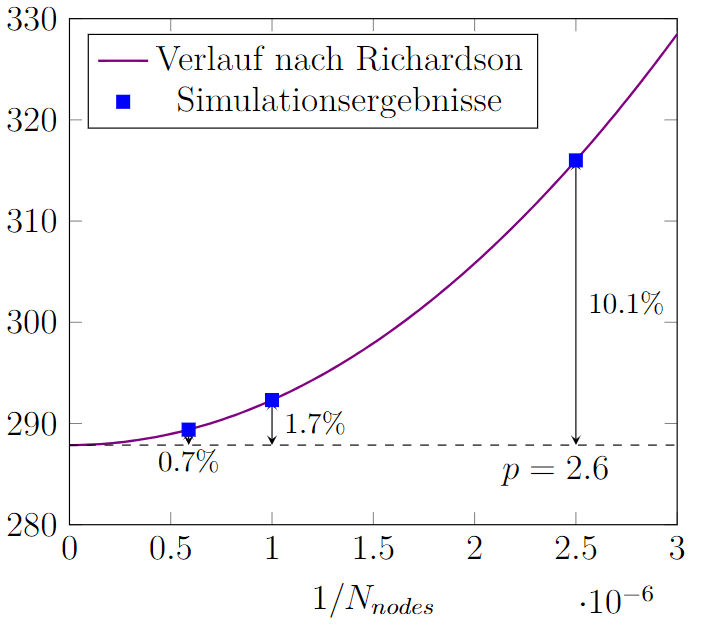
Before trusting any result, the mesh had to earn it. We ran the model on three refinement levels and applied Richardson extrapolation — the 1927 'deferred approach to the limit' — to estimate the grid-independent solution and the observed convergence order, which came out at p ≈ 2.6.

Against the extrapolated limit, the coarse mesh sat 10.1 % off, the medium mesh 1.7 %, the fine mesh 0.7 %. The medium mesh became the workhorse for everything that follows: within two percent of converged, at a fraction of the fine mesh's solve time — a relevant trade when the dynamic runs ahead would need thousands of time increments.

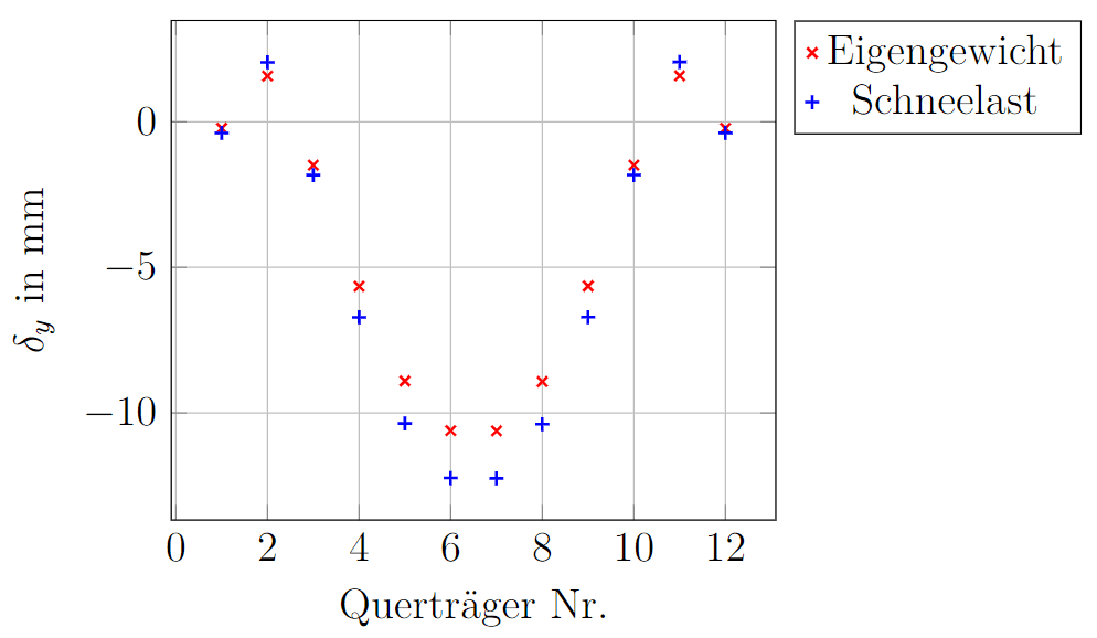
As a static sanity check, the model was also put through classic load cases — self-weight and snow load — giving mid-span deflections of around a centimetre, symmetric across the twelve cross-girders, exactly the order of magnitude one expects from a 15-tonne steel span.

The eigenfrequency computation has one subtlety that dominates everything: the X-cables only stiffen the bridge because they are pre-tensioned. So the analysis runs in two steps — a geometrically nonlinear static step (NLGeom) applies the pre-tension and updates the stiffness matrix, and only then does the frequency step extract the modes on that stressed configuration. Skip that, and the frequencies come out wrong by double-digit percentages.

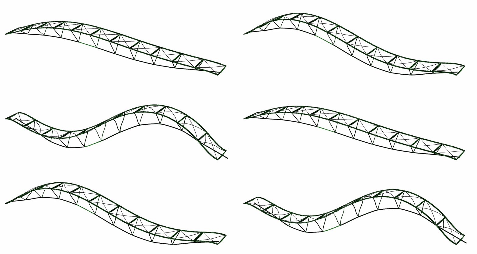
The first eigenmode appears at 1.98 Hz — a horizontal sway of the whole deck, the kind of mode wind or lateral crowd motion would excite. The second, at 2.10 Hz, is the one that matters for a footbridge: a vertical oscillation straight in the direction of pedestrian loading. Above those two, the spectrum fills in at 2.70, 3.14, 3.66 Hz and onwards, with a dense cluster between 5.8 and 6.2 Hz.

And the number from the 1999 journal? Measured second eigenfrequency: about 2.1 Hz. Simulated: 2.0985 Hz. Twenty-five years between the measurement and the model, and the modal analysis lands on it almost exactly — the first strong sign the model was capturing the real structure.

With a validated modal model, we started turning knobs. Remove the cable pre-tension and the spectrum collapses: the first mode drops from 1.98 Hz to 1.09 Hz and the mode shapes reshuffle entirely — the cables' geometric stiffness is not a correction, it is the design. Cool the bridge by 30 °C and the frequencies climb by roughly 5–7 % from thermal contraction alone, and by around 11 % once the contraction's extra cable tension is included. Adding damping, by contrast, shifts the eigenfrequencies not at all — exactly as theory promises for a lightly damped structure.

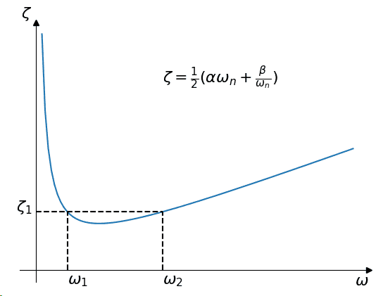
Damping itself needed a decision. Fifteen tonnes of welded steel means very little inherent energy dissipation — light and lightly damped is precisely the combination that makes footbridges vibration-prone. Since the load cases of a bridge are strongly frequency-dependent, we chose Rayleigh damping: the α/β coefficients are fitted so the damping ratio ζ is correct at two anchor frequencies, giving a physically sensible ζ across the band where the bridge actually responds.

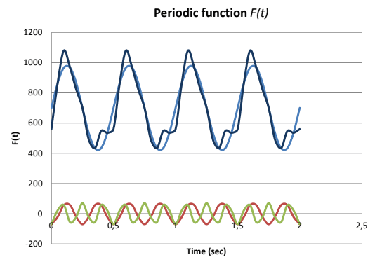
To shake a bridge in simulation you first need a credible human. Footfall forces are well studied: a walking pedestrian loads the deck with their static weight plus periodic harmonics of the step frequency. Following the literature model, we built F(t) = G₀ + G₁·sin(2πf·t) + Σ Gᵢ·sin(2πif·t − φᵢ): a static component of about 700 N, a first harmonic at 40 % of body weight, and second and third harmonics at 10 % each with phase shifts.

The resulting force history was validated against the published curves, then distributed over the deck as the moving crowd load for the dynamic runs. Two Abaqus solution strategies were set up side by side: Modal Dynamic — time integration on the modal basis, cheap enough for long load histories — and Steady-State Dynamic, which solves the frequency response directly and answers 'what if the crowd walks at exactly this rate?' for every frequency at once.

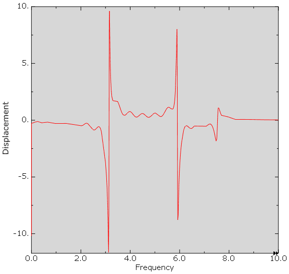
The steady-state sweep from 0 to 10 Hz makes the modal analysis visceral: sharp displacement peaks rise at 3.14 Hz and 5.9 Hz — the vertical modes that a deck-distributed load actually projects onto. The horizontal first mode at 1.98 Hz is invisible to a purely vertical pedestrian load, exactly as it should be.

Then the same story in the time domain: harmonic excitation at three frequencies. At 2 Hz the bridge responds but stays civilised. At 3.14 Hz — dead on the resonance — the amplitude grows cycle by cycle into by far the largest response of the study. At 10 Hz, far above the relevant modes, the deck barely notices the load at all. Three animations, one lesson: it is not the size of the force but where it sits in the spectrum.

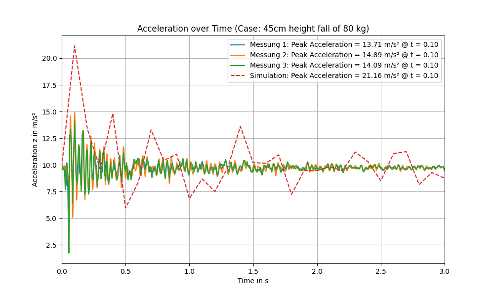
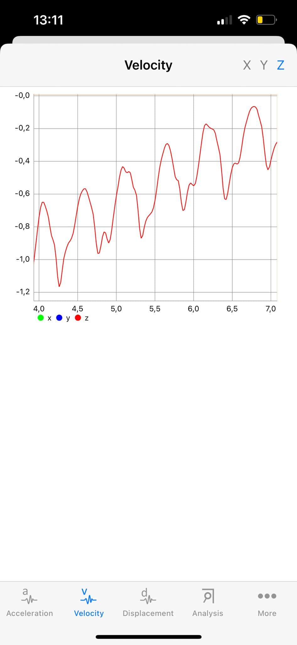
The best part of modelling a bridge you walk past every week: you can go and test it. For the spontaneous-excitation load case, one of us jumped on the deck while a smartphone accelerometer lay on the walkway recording the decay — three repetitions, peak vertical accelerations between roughly 13.7 and 14.9 m/s², and a beautifully clean dominant frequency of 1.95 Hz in the free vibration afterwards. Simulated second eigenmode: 2.10 Hz. A phone on a footbridge confirming a quarter-century-old journal measurement and an Abaqus model at the same time.

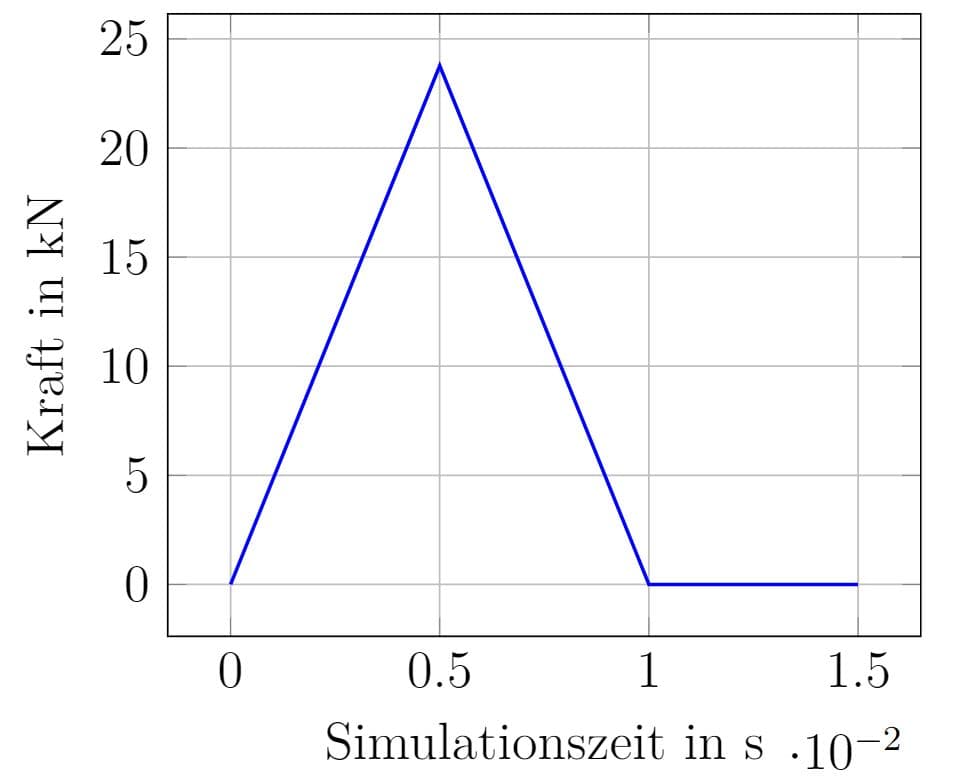
On the simulation side, the jump became a triangular force impulse — ramping to 24 kN and back to zero within 10 ms at the jump position — followed by a modal-dynamic free decay with the Rayleigh damping from chapter 05. Same bridge, same spot, same physics: one history measured, one computed.

Overlaying simulation on the three measured decays gives the honest final picture. The frequencies match convincingly — the simulated response oscillates at the same rate as the measured one, which is the modal model doing its job. The amplitudes don't: the simulation peaks at 21.2 m/s² against roughly 14 m/s² measured, and its low-frequency content rings noticeably longer than reality.

The diagnosis wrote itself into the discussion section. The Rayleigh α coefficient — the term that damps low frequencies — was chosen too small, and the model contains no structural or friction damping at all: every bolted joint, bearing and micro-slip mechanism in the real bridge dissipates energy the model doesn't know about. On the amplitude side, the idealised point-impulse force introduction, the simplified geometry and the assumed boundary conditions all push in the same direction.

Which is the right ending for a semester of FEM: a model that nails the spectrum — meshed, converged, prestressed and benchmarked against two independent measurements — and a validation experiment that shows precisely where the modelling assumptions stop being free. The frequencies are physics; the damping, as always, is the confession.