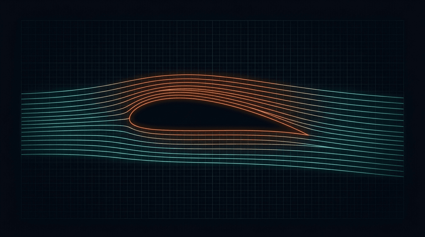
Custom 2D Airfoil Design Code
An inverse 2D airfoil design tool: prescribe the velocity distribution and get the geometry plus its full polar — exact potential-flow core, integral boundary-layer analysis with transition prediction, and an interactive GUI. Prototyped in Python, final version in C++.
The pressure distribution is the real design object — not the shape
Ask what makes a wing section good and the answer is never really the shape itself. It's what the flow does over it: where the air accelerates, how long the boundary layer stays laminar, how gently the pressure recovers towards the trailing edge, whether the flow stays attached at high lift. All of that is written into one curve — the velocity (or pressure) distribution along the surface.
Most tools attack the problem the obvious way round: draw a shape, analyse it, look at the distribution, tweak the shape, repeat. This project takes the opposite route. You prescribe the velocity distribution you want the airfoil to have, and the code computes the unique geometry that produces it. The shape falls out as a consequence of aerodynamic intent, not the other way round.
The goal was a complete, self-contained 2D airfoil design environment: an inverse design core, a boundary-layer analysis that predicts transition, separation and drag, and an interactive GUI that turns the whole thing into a live design loop — move a slider, get a new airfoil and its full polar seconds later.
Why design backwards?
The direct route — geometry in, pressures out — is an analysis method pressed into service as a design method. It works, but every iteration is guesswork: thickening the nose to soften a suction peak also moves the peak, changes the recovery, shifts transition. The designer is steering through the geometry, one step removed from the quantity that actually matters.
Inverse design removes that indirection. Laminar flow is wanted over the front 40% of the upper surface? Then prescribe a gently accelerating velocity there — a favourable pressure gradient holds the boundary layer laminar almost by definition. The recovery region should avoid separation? Choose a recovery shape that stays safely below the separation criterion. Each aerodynamic requirement maps directly onto a feature of the prescribed distribution, and the geometry that results is, by construction, the section that meets it.
The catch is mathematical: not every velocity distribution corresponds to a physically valid, closed airfoil. Handling that constraint properly — rather than hoping — is where most of the theory in this project lives.
Choosing the right level of physics: incompressible potential flow
Full viscous flow is governed by the Navier–Stokes equations — accurate and, for a fast design loop, hopelessly expensive. Dropping viscosity gives the Euler equations. But for an airfoil well below stall one can go a step further: outside the paper-thin boundary layer the flow is not only effectively inviscid but also irrotational, and at low Mach numbers incompressible. Under those three assumptions the whole flow field reduces to a single linear equation — Laplace's equation for the velocity potential.
That reduction is what makes the method fast and, more importantly, exact: potential flow around a 2D body can be solved in closed form, with no grid, no discretisation error and no turbulence model in the outer flow. The price is equally clear, and it defines the honest operating envelope of the code: strictly incompressible (trustworthy up to roughly Mach 0.3, stretchable with a compressibility correction, never transonic — no shocks, no wave drag) and inviscid in the outer field, so all viscous physics has to be reintroduced separately through a boundary-layer model.
Viscosity, though, is exactly where drag, transition and stall live. So the architecture is a classic two-layer one: an exact potential-flow solution for the pressure field, coupled to an integral boundary-layer method that runs along the surface afterwards. Chapters 08–10 cover that second layer.
Solving the flow exactly by mapping a circle
The classical trick for exact 2D potential flow: the flow around a circle is known analytically, and any smooth airfoil-like contour can be related to a circle by a conformal map — an angle-preserving transformation of the complex plane. Map the circle solution through that transformation and you have the exact flow around the airfoil, at any angle of attack, including the circulation that sets the lift via the Kutta condition at the trailing edge.
For inverse design this becomes even more elegant. Points on the circle are identified by their polar angle ν, running from 0° at the trailing edge over the upper surface to 360° back at the trailing edge. The designer prescribes the velocity as a function of ν, and the mapping that turns the circle into the airfoil is derived from that prescription — the surface velocity distribution and the geometry are two faces of the same analytic function.
Working in the circle plane also solves a practical annoyance for free: points equally spaced in ν crowd together near the leading edge in the airfoil plane, exactly where the curvature is highest and resolution is most needed. The 66-point contour the code outputs is dense at the nose and coarse on the flat parts without any explicit grading logic.
Segments and design angles: one α* per stretch of surface
Prescribing a raw velocity curve point by point would be clumsy and would almost never satisfy the closure constraints. Instead, the front part of the airfoil is described segment by segment, and each segment is given a design angle of attack α* — the angle at which the velocity over that segment is exactly constant.
That indirection is the key idea of the whole parametrisation, because a constant velocity at α* means something precise for the boundary layer: below α* the segment sees a favourable (accelerating) gradient, above it an adverse one. Assigning α* = 7° to the forward upper surface says: keep this region laminar-friendly for all angles up to 7 degrees. Choosing a sequence of slightly increasing α* values towards the nose builds in graceful off-design behaviour — as incidence rises, the adverse gradient creeps forward smoothly instead of a suction spike appearing at once.
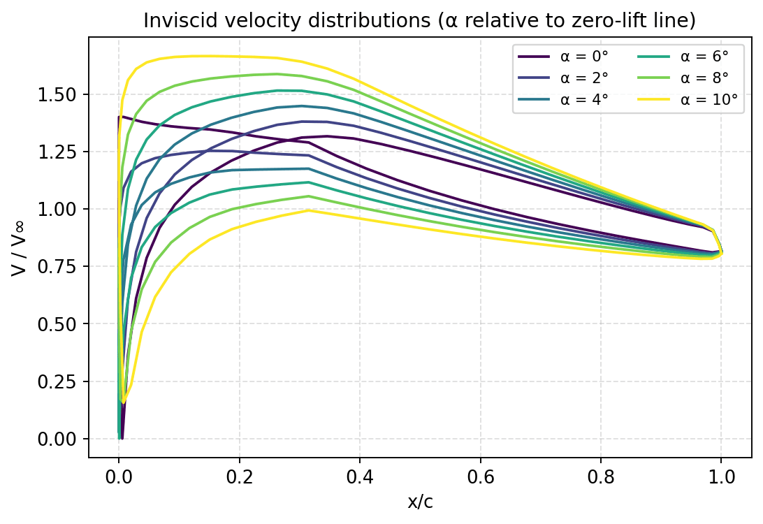
In effect, the designer specifies the polar, not the shape: which range of lift coefficients each part of the surface should serve. The upper surface is designed at the top of the intended low-drag range, the lower surface at the bottom. The velocity distributions below — computed for angles from 0° to 10° relative to the zero-lift line — show the result: a wide fan of distributions from a single geometry, with the front-loaded acceleration regions doing exactly what their design angles promised.
λ, μ, ω — three numbers that shape the aft airfoil
Aft of the design segments the flow has to slow back down towards the trailing edge — the pressure recovery. This is the most delicate region of any airfoil: recover too aggressively and the turbulent boundary layer separates; recover too timidly and the airfoil ends up thin and the forward surface can't carry low pressure for long. The code parametrises the recovery with three numbers per surface.
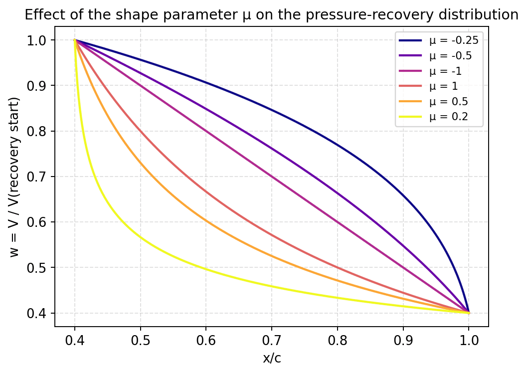
λ (lambda) sets where the recovery begins and how much arc it occupies — effectively the extent of the recovery region. μ (mu) sets its shape, blending continuously between a concave, gentle-at-first recovery (negative μ) and an aggressive, front-loaded one approaching a Stratford-like distribution that flirts with separation everywhere at once (small positive μ). ω (omega) blends in the closure contribution near the trailing edge — the final steep bit of recovery that guarantees the contour actually closes.
These six values — λ, μ, ω for each surface — are the main design freedoms once the segment structure is fixed, and they became the primary sliders in the GUI. The figure shows the μ family: every curve recovers the same total velocity ratio, but distributes the adverse gradient completely differently along the surface.
Not every wish list is an airfoil
Here is the mathematical heart of inverse design: a prescribed velocity distribution is only realisable if it satisfies three integral constraints. The mapping must return to its starting point (two conditions, one per coordinate — otherwise the 'airfoil' is an open spiral), and the flow far away must reduce to a clean uniform stream. Prescribe velocities freely and all three will, in general, be violated.
The code therefore treats a handful of the prescribed quantities not as user inputs but as unknowns — among them the closure contributions controlled by ω and an auxiliary constant K_S — and solves a small system of transcendental equations so that the constraints come out exactly. This is done with an iteration that typically converges in three to five steps, after which the design angles are re-normalised (which is why the α* values shift slightly between the first and the converged pass).
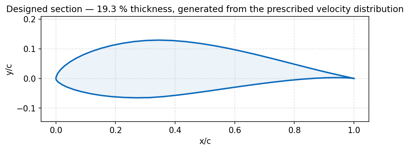
It's a genuinely satisfying piece of numerics to watch: the residual K_S drops from order one to below the rounding threshold in four iterations, and out comes a closed contour — in the example run, the 19.3%-thick section shown in chapter 01, with its zero-lift angle (4.27°) and zero-lift pitching moment (−0.101) delivered as by-products of the same solution.
An integral boundary-layer method along the surface
The potential-flow solution knows nothing about drag — d'Alembert's paradox guarantees it. All viscous physics is confined to the boundary layer, and because that layer is thin, it doesn't need a 2D flow solver of its own: its state at each surface station can be summarised by a few integral thicknesses, and their evolution follows ordinary differential equations driven by the outer velocity distribution.
Concretely, the method marches from the stagnation point along each surface, integrating the momentum-integral equation (von Kármán) together with an energy-integral equation. Two quantities carry the state: the momentum thickness, which measures accumulated momentum loss, and the shape factor built from the energy and momentum thicknesses, which measures how 'healthy' the velocity profile is. Laminar and turbulent stretches use different closure relations for skin friction and dissipation, calibrated against classical boundary-layer data.
Because the boundary layer is fed directly by the designed velocity distribution, cause and effect stay legible: steepen the recovery with μ and you watch the shape factor dive towards its separation limit; extend a favourable gradient with a higher α* and transition walks aft. This tight coupling between the design parameters and the boundary-layer response is what makes the tool educational rather than a black box.
Predicting where laminar flow ends — and what it costs
The single most consequential event in the boundary layer is transition. A laminar layer has a fraction of the skin friction of a turbulent one, so every millimetre of laminar run pays directly into the drag budget; but a laminar layer is also fragile, separating under adverse gradients a turbulent layer would shrug off. The code predicts natural transition with an empirical criterion based on the local momentum-thickness Reynolds number and the shape factor: healthier profiles (favourable gradients) tolerate a higher Reynolds number before transitioning, while decelerating profiles trip early.
Laminar separation gets special treatment. If the laminar layer separates before the transition criterion is met — typical at moderate Reynolds numbers when the recovery starts too abruptly — the code flags a laminar separation bubble: the separated shear layer transitions in mid-air, and the now-turbulent flow usually reattaches, at the cost of extra drag and, in bad cases, hysteresis. Rather than resolving the bubble, the method flags it and adds an empirical drag penalty — and, more usefully, gives the designer the tool to avoid it: a short, mildly destabilising 'ramp' region ahead of the main recovery that coaxes the boundary layer through transition before the steep gradient hits. The ramp length and depth are two further sliders in the GUI.
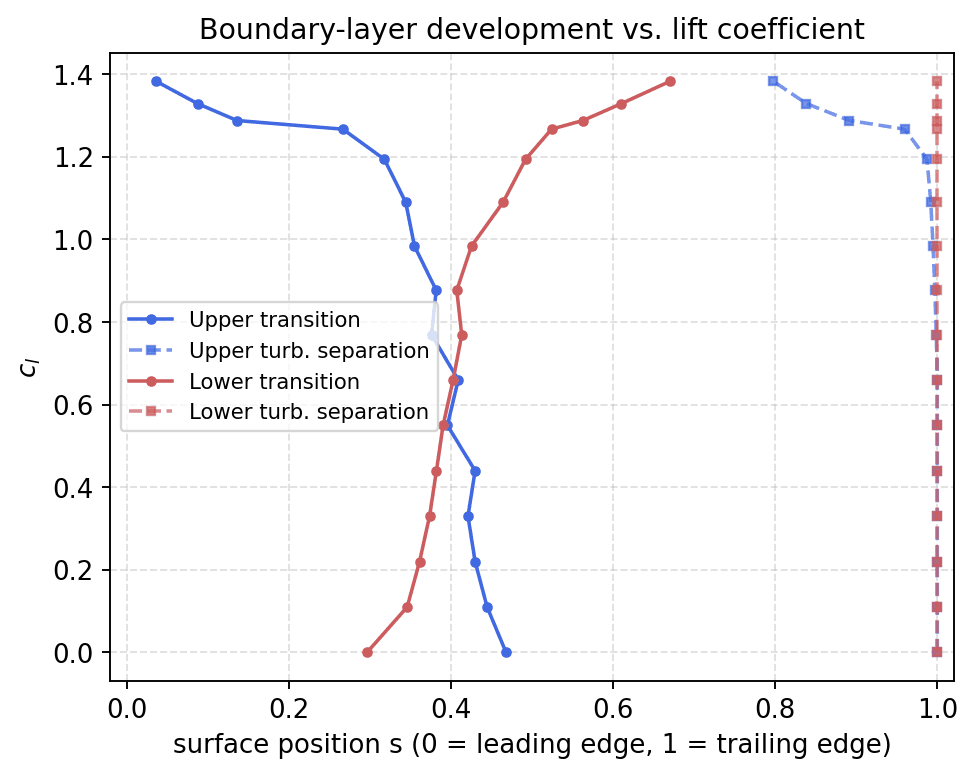
Turbulent separation is monitored the same way, via the shape factor. The plot shows the whole story at a glance for the example section: transition (solid) marching forward on the upper surface as lift increases, aft on the lower surface, with turbulent separation (dashed) pinned at the trailing edge until the highest lift coefficients — precisely the behaviour designed in.
Drag from the wake: the Squire–Young extrapolation
With the boundary layer integrated to the trailing edge, drag follows from momentum accounting. Far downstream, the profile drag of the section equals the momentum deficit carried by the wake — but the boundary-layer solution stops at the trailing edge, where the deficit hasn't finished developing. The classical bridge is the Squire–Young formula: it extrapolates the momentum thickness at the trailing edge to the far wake, using the local trailing-edge velocity and an assumption about how the wake relaxes towards freestream pressure.
Upper and lower surface each contribute their share; the bubble penalties from chapter 09 are added on top. Lift and pitching moment come from the potential-flow circulation, corrected for the boundary layer's decambering effect — the displacement of the outer flow slightly de-loads the aft airfoil, which is why the delivered lift-curve slope sits below the ideal 2π and why the code applies a lift-efficiency correction rather than reporting bare inviscid values.
None of this is exotic — these are the standard tools of classical airfoil analysis — but implementing them yourself, and watching the drag polar respond to a single slider nudge in the recovery shape, teaches more section aerodynamics than any number of canned CFD runs.
From one geometry to a full polar in about a second
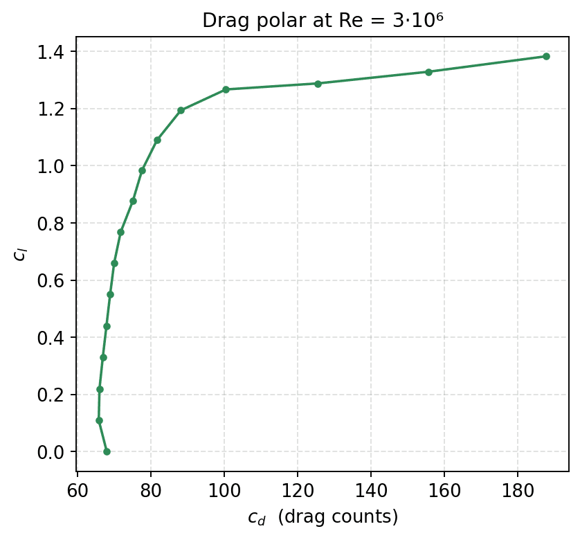
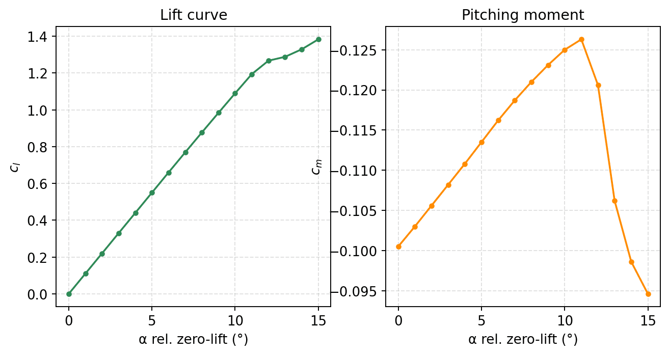
A design run produces everything needed to judge a section: the geometry itself, velocity distributions at any set of angles, and a complete polar — lift, drag and pitching moment across the operating range, with transition and separation positions logged for every point. The example below is the 19.3% section at a Reynolds number of 3 million, analysed from 0° to 15° relative to the zero-lift line.
The polar shows the signature of a laminar section: a low-drag bucket (here around 65–70 drag counts) spanning the lift range the design angles were chosen for, with drag rising steeply once transition reaches the nose and the upper-surface bubble warnings accumulate above cl ≈ 1.2. The moment curve stays flat near −0.10 to −0.12 until trailing-edge separation begins to unload the aft camber at the top of the range — visible as the hook back towards zero.
Reading these three plots together — and understanding why each feature traces back to a specific design parameter — is the entire craft of section design, compressed into one screen.
Turning a batch solver into a live design loop
The numerical core alone is a batch program: edit a text input file, run, read a few hundred lines of tabulated output. Usable, but it throttles exactly what inverse design is good at — rapid, intuition-building iteration. So the second half of the project was wrapping the solver in a GUI that closes the loop.
The interface exposes the aft-design parameters as sliders — λ, μ, ω for each surface, plus the two ramp controls — and one button: run. On each run the tool writes the parameters into the input file, executes the solver, parses the full output, and refreshes four linked plots: velocity distributions, lift curve with transition/separation overlay, moment curve, drag polar — plus a live preview of the section itself. Standard file handling (new/open/save/save-as, modified-state tracking), persistent settings and a dark mode round it off.
The whole cycle takes about a second, and that speed changes how the tool is used. Sweeping μ from −0.5 to +1 in ten steps and watching the polar's low-drag bucket widen, shift and finally collapse into separation teaches the recovery trade-off viscerally — the kind of understanding that batch runs with minutes of turnaround never produce.
Prototype in Python, production in C++
The first complete version was Python: the numerics prototyped where they're quickest to get right, the interface in Tkinter with embedded Matplotlib figures, pandas doing the output wrangling. Python was the right choice for working out the method — every intermediate quantity is one print statement away, and refactoring the parametrisation cost minutes instead of hours.
For the final version the code moved to C++. Partly for raw speed — parameter sweeps and future optimisation loops want the solver call to be milliseconds, not the better part of a second — and partly for robustness: a compiled, statically-typed numerical core with no interpreter and no dependency environment is simply a nicer thing to ship and to keep working years later. The Python version survives as the reference implementation the C++ results were validated against, which proved its worth more than once when a subtle indexing bug in the port produced polars that were almost, but not quite, right.
The two-stage approach is one of the main process lessons of the project: prototype the physics in the language where thinking is cheap, port to the language where running is cheap, and keep the prototype alive as the ground truth.
A surprising amount of real aerodynamics for a 1-second computation
It's worth being precise about what physics is actually in the loop. Captured: the exact inviscid pressure field at any incidence, including the correct nonlinear behaviour near the leading edge that thin-airfoil theory misses; laminar and turbulent boundary-layer growth driven by that field; natural transition as a function of Reynolds number and pressure-gradient history; laminar separation bubbles (flagged, with empirical drag penalty); turbulent trailing-edge separation onset; profile drag from the wake momentum deficit; lift and moment including the boundary layer's decambering correction; and the dependence of all of the above on Reynolds number.
That list covers the phenomena that dominate section behaviour for essentially the whole low-speed envelope — sailplanes, propellers, UAVs, wind-turbine blades, general aviation. It's the same modelling level that generations of proven laminar airfoil families were designed with, which was exactly the ambition: not a toy, but the real classical toolchain, built end to end.
Knowing exactly where the code stops being trustworthy
Every simplification in chapter 03 has a bill attached, and part of the project was learning to state it precisely. Compressibility: the flow model is strictly incompressible. Below Mach ≈ 0.3 the error is negligible; towards Mach 0.5–0.6 a Prandtl–Glauert or Kármán–Tsien correction could stretch the pressure predictions, but the moment the local flow goes supersonic the model is silently, fundamentally wrong — no shocks, no wave drag, no drag divergence. Transonic design is out of scope by construction, not by tuning.
Viscous coupling: the boundary layer listens to the potential flow, but the potential flow never hears back (beyond the global decambering correction). This one-way coupling is accurate while the layer stays thin and attached — and progressively fiction once significant separation develops. Consequently the code cannot predict maximum lift or stall shape; it can only warn where separation begins. Bubbles are flagged and penalised, not resolved, so at low Reynolds numbers (below roughly 10⁵, where bubbles dominate) the drag numbers become qualitative. Transition is an empirical correlation, valid for smooth surfaces in low-turbulence flow — roughness or a dirty environment shifts it in reality but not in the model, except by forcing transition manually.
And structurally: everything is 2D, steady and single-element. No sweep, no finite-wing effects, no flaps in the model, no unsteady aerodynamics. None of these limits is a flaw — each is the direct price of the one-second design loop — but the difference between a dangerous tool and a useful one is that the boundaries are known, stated, and respected.
The fastest way to learn aerodynamics is to build the tool
The project delivered exactly the intuition it was started for. Concepts that stay abstract in lectures — why a favourable gradient delays transition, why an aggressive recovery buys thickness but risks the bucket, why moment and camber trade against each other, why low-Reynolds sections need their recovery softened — became things felt through the sliders, because every one of them is a visible cause-and-effect in the four plots.
It also sharpened engineering judgement about models in general: an exact solution of the wrong equations (pure potential flow) is useless for drag, while a stack of well-chosen approximations — integral boundary layer, empirical transition, wake extrapolation — predicts real polars remarkably well inside a known envelope. Fidelity is not one number; it's an itemised list.
A foundation for optimisation
With a solver call this cheap, the natural next step is to stop moving the sliders by hand: wrap the design loop in an optimiser and search the λ–μ–ω–α* space directly against polar objectives — widest bucket at a target cl, best endurance figure of merit, mildest moment. A compressibility correction for the high-subsonic end and a proper bubble drag model for the low-Reynolds end are the two most valuable physics upgrades on the list.
The code has already earned its keep beyond its own page: it became the workhorse behind the Horten H3 airfoil modernisation project, where the design loop ran against a historic flying wing's stability constraints. That's the quiet test of a self-built tool — whether it gets reached for when the next real problem shows up.